Introduction

In this post, I’ll show you how you can create a gradient from a 2D SDF and how it can be used as a flowmap in the material to warp a texture or in Niagara to drive the location of particles! I’ve also added a bonus section about Anti Aliasing, something that I haven’t covered before.
If you haven’t seen my previous posts about SDF I highly recommend them:

1. Basic Shapes and Visualization
2. Combine Shapes
3. Manipulate Space

Gradient / Flowmap

Shape

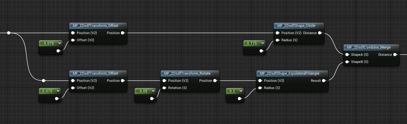
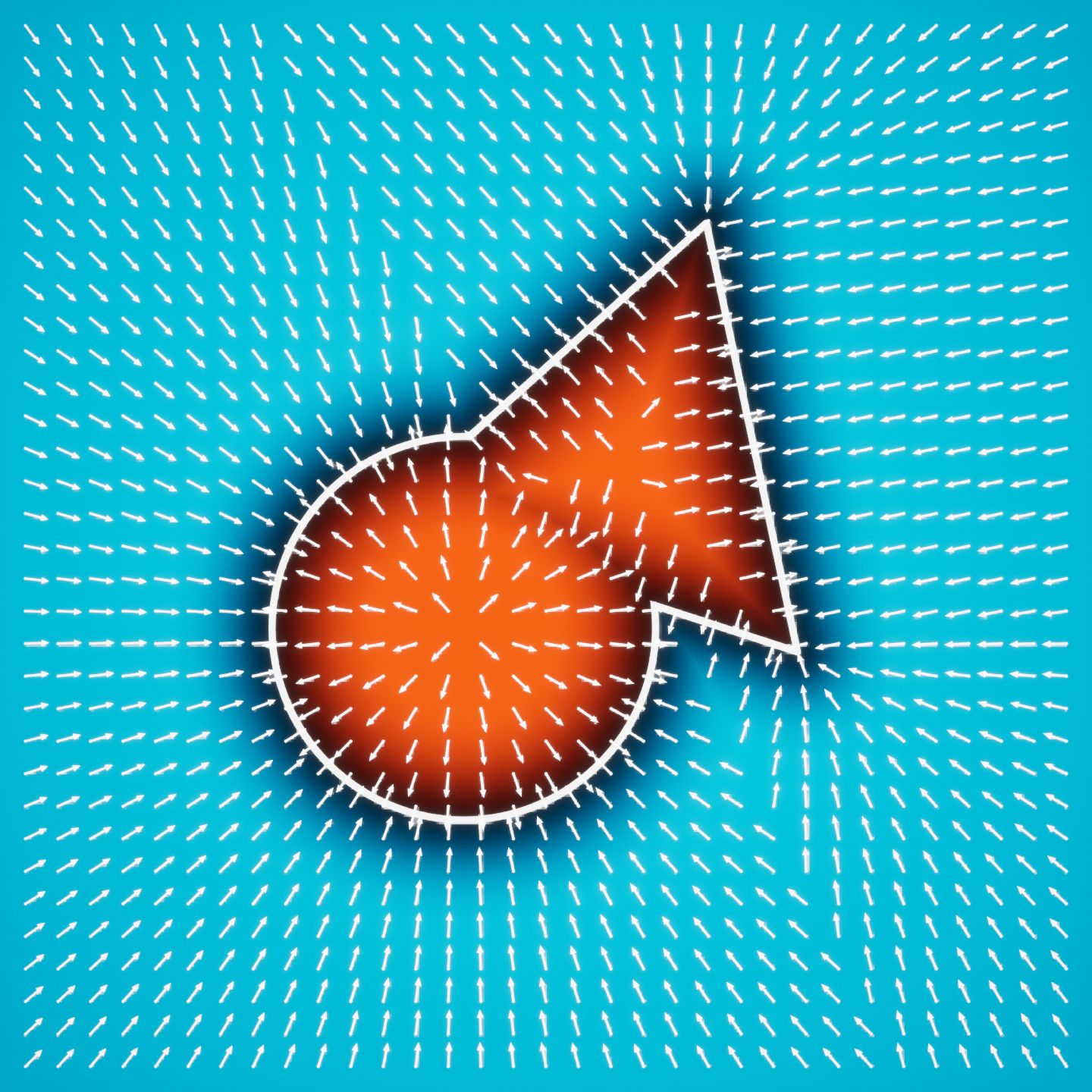
For the rest of the post I will use an SDF of a sphere and a triangle combined together that looks like this:

Here’s the graph, you can find how to create these functions in my previous posts:

Explanation

For understanding how to make gradients form SDFs I’ve read this post, have a look at it if you want some more in detail explanation.

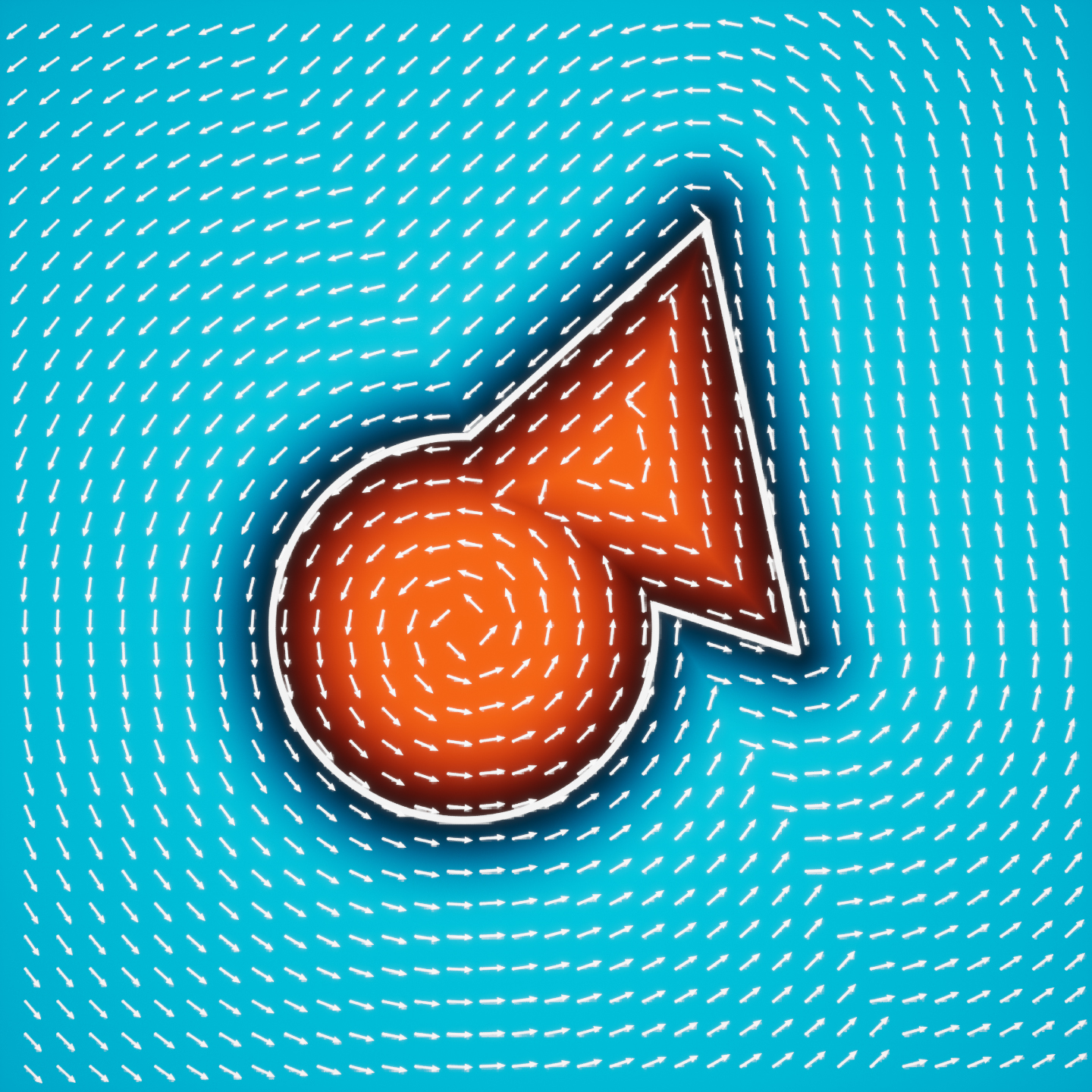
If you’ve read my first post about SDFs it’s probably you should know that each point in the field of an SDF stores the distance to the closest edge of the shape, we can use this information to calculate a gradient, which will be a direction that points either directly towards or away from the closest edge. This is done by comparing the value of each point in the field to the value of their neighbors on the X and on the Y axes.

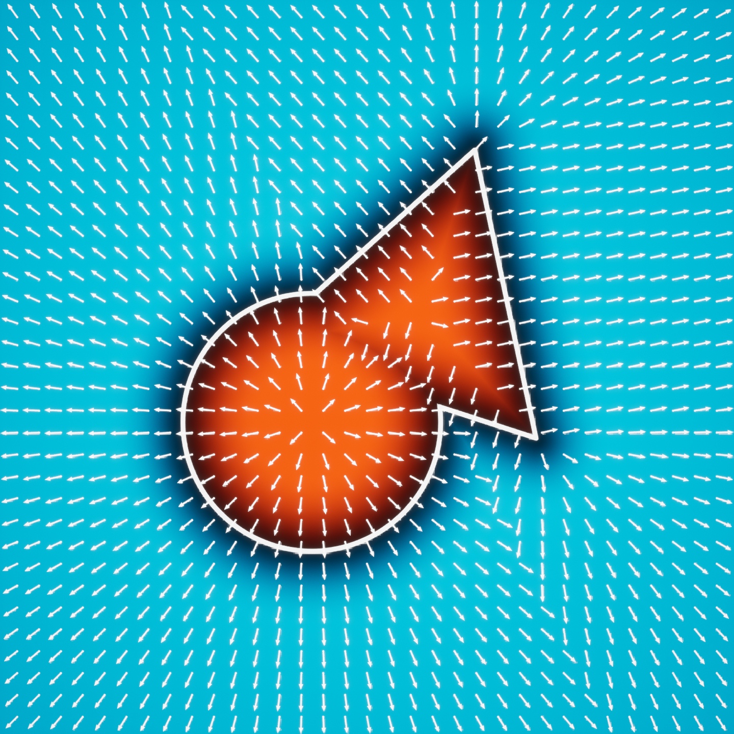
The arrows in the image above show the gradient.
Inside the field, where the distance is negative, the gradient points directly towards the edge.
Outside it, the gradient points directly away from the edge.
These directions can be expressed as a 2D vector, which is referred to as the gradient vector.

Logic

The only thing to keep in mind is that this gradient doesn’t come cheap, to generate it we need to sample the sdf two extra times, with some offset on the X and on the Y to calculate the derivatives of the two axes. This just means that we need the change of rate in both X and Y.

Because we need to sample the SDF three times I would highly recommend creating a Function that contains the shapes of the SDF you are working on, especially if you’re manipulating and combining multiple shapes.

We first need to sample the distance as usual, then to calculate the change of rate in the X axis we need to add a slight offset on the position and then sample the SDF again, this way we are essentially finding the Right Neighbour value for each point in the SDF. Then subtracting it from the distance calculated earlier, we get the change of rate on X. We can do the same for getting the Top Neighbour of the SDF and the change of rate in Y.
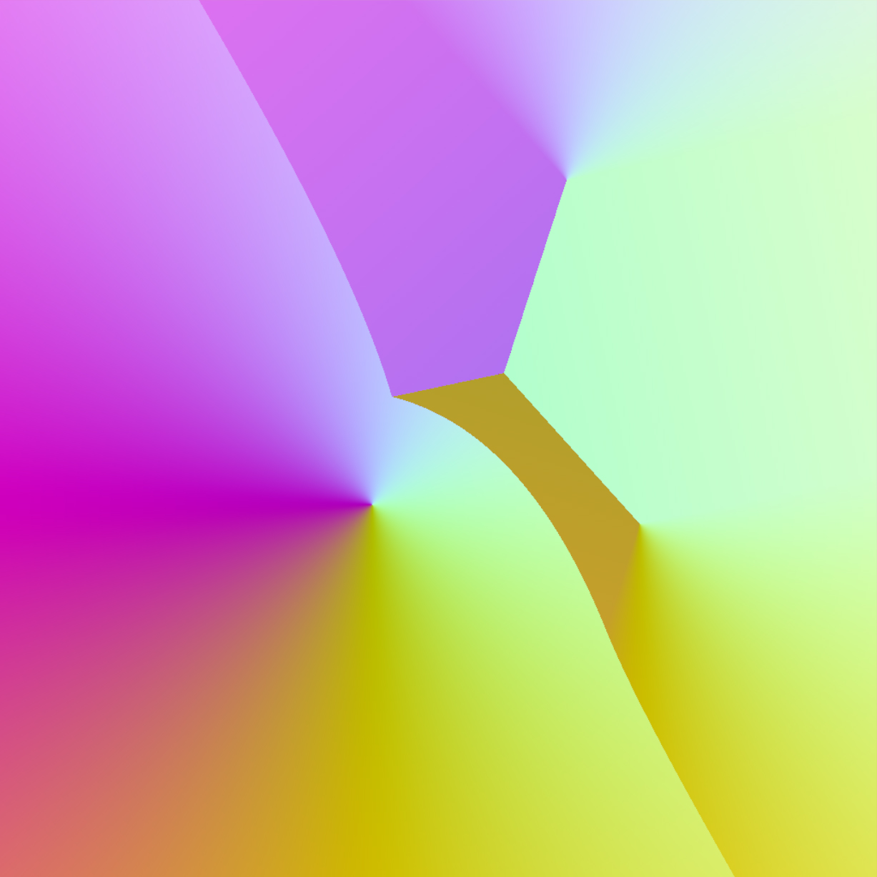
If we then make a Vector2 appending the two results and normalize it, we get the gradient.

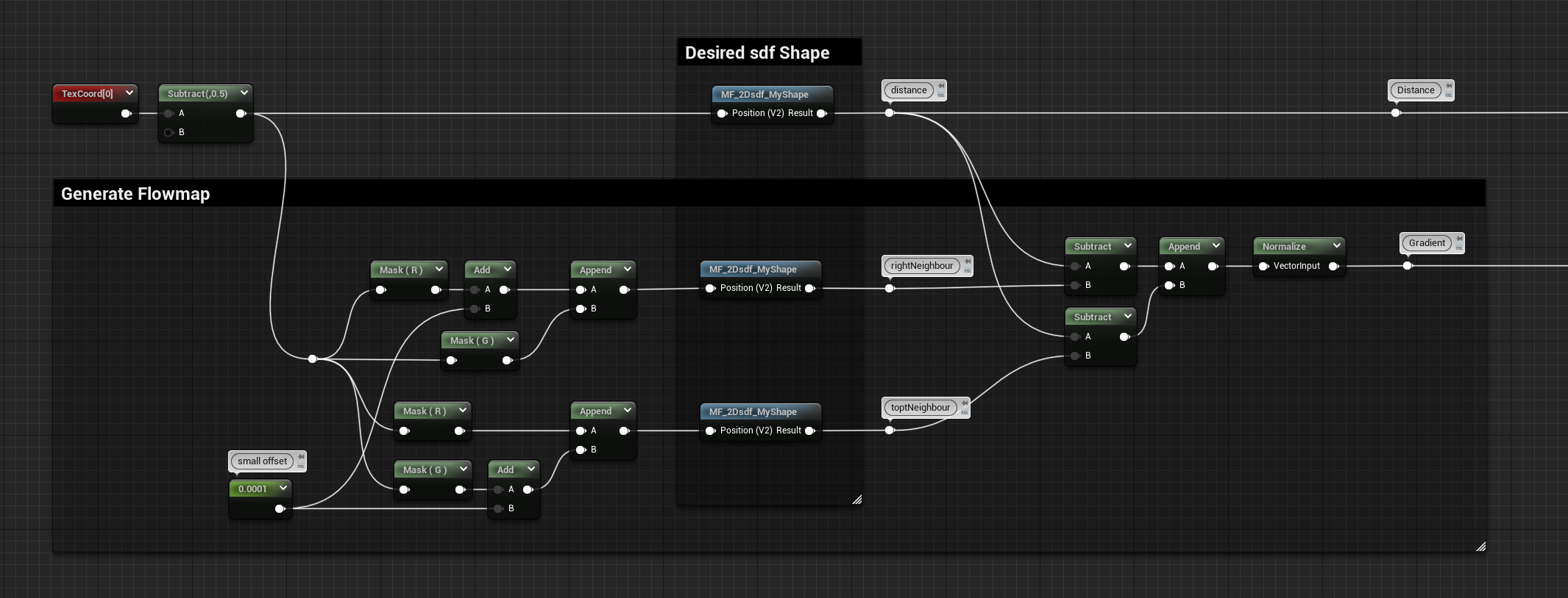
And here it is in all its glory:

Warp Texture

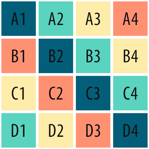
This gradient can be used as a flow map to warp and distort textures, for my examples I will be using this texture with some tiling:

For demonstration purposes, I’ve only set up a simple example.
You can multiply the gradient to control the strength of the warp, then multiply again with Time and add it to the UVs of your texture. I’m also controlling the speed multiplying Time and I’m feeding it to a Frac node to have the distortion happen in a repeating loop:

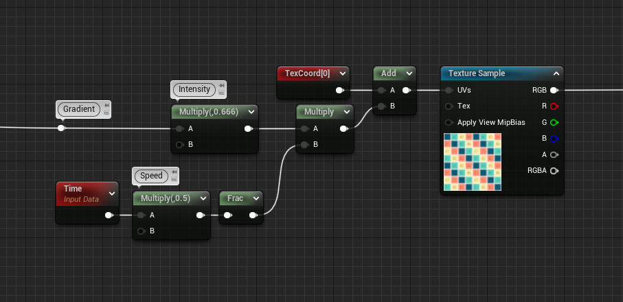
You can see that the texture will move outward from the center of the SDF, just like the direction of the arrows shown earlier:

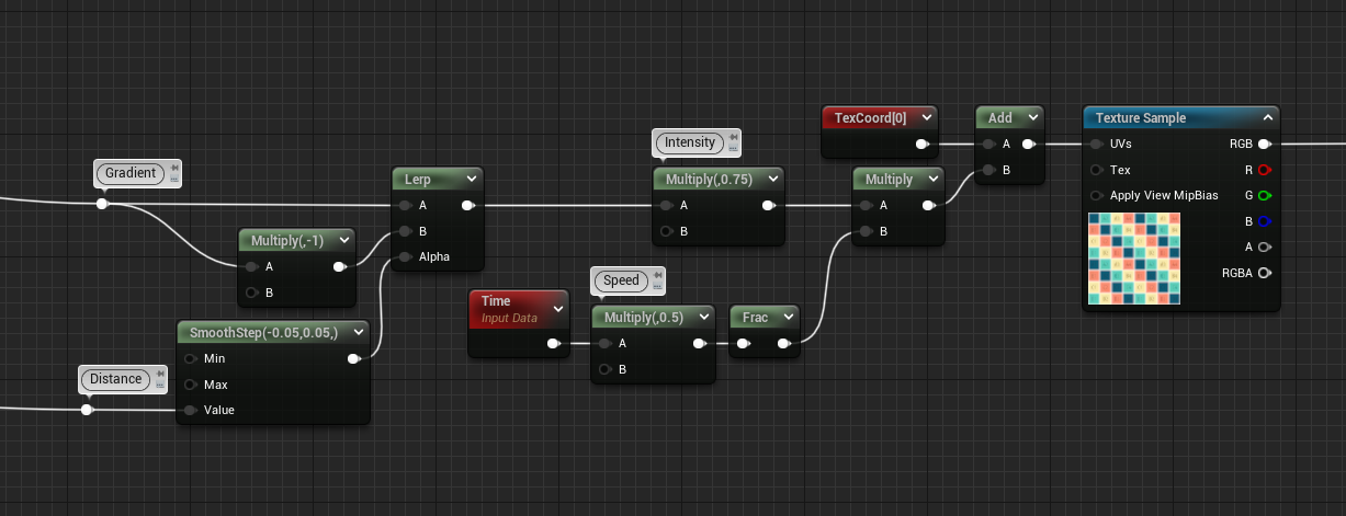
Of course, we can mask this distortion using the distance value of the SDF, in the example below I’m inverting the direction of the flow for everything that is outside of the shape and keeping it the same as before for the inside. This can be easily done with a Lerp node, in this case, I’m also using a Smooth Step function to remap the SDF (again, more about this in my previous posts)

Render Target

What’s cool is that we can draw both the distance and the gradient of the SDF to a Render Target and read the texture in Niagara to control the location and low of particles!!

When drawing the Material to a Render Target we need to keep in mind that we can only have values in the range of 0 to 1. However, we know that the distance of the SDF contains negative values for the points inside the shape and the directions of the gradient also contain some negative values. So we need to lift them all to be in the range needed, this can simply be done by adding 1 and multiplying by 0.5.

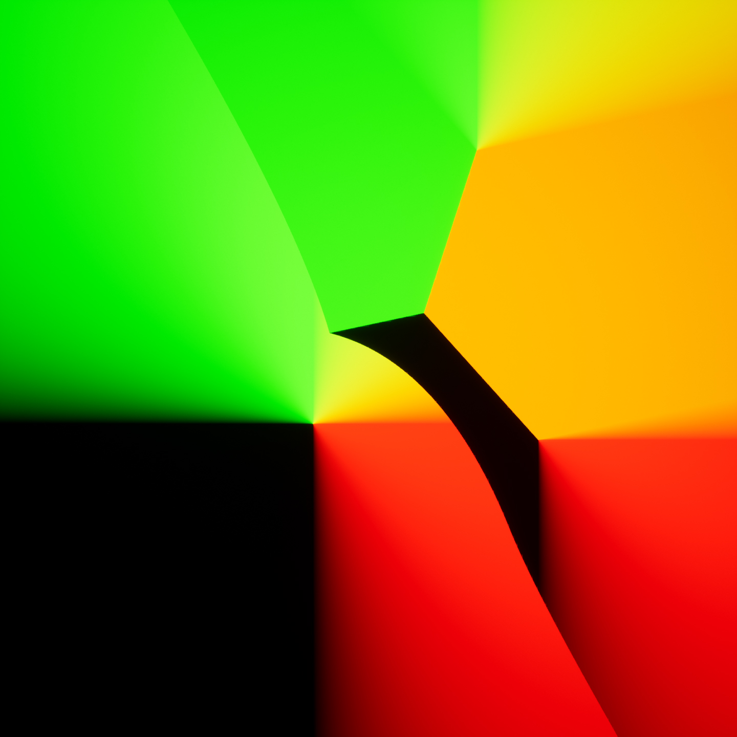
What I also like to do is to combine them both in a vector3, having the distance in the Red Channel and the gradient in the Green and Blue ones.

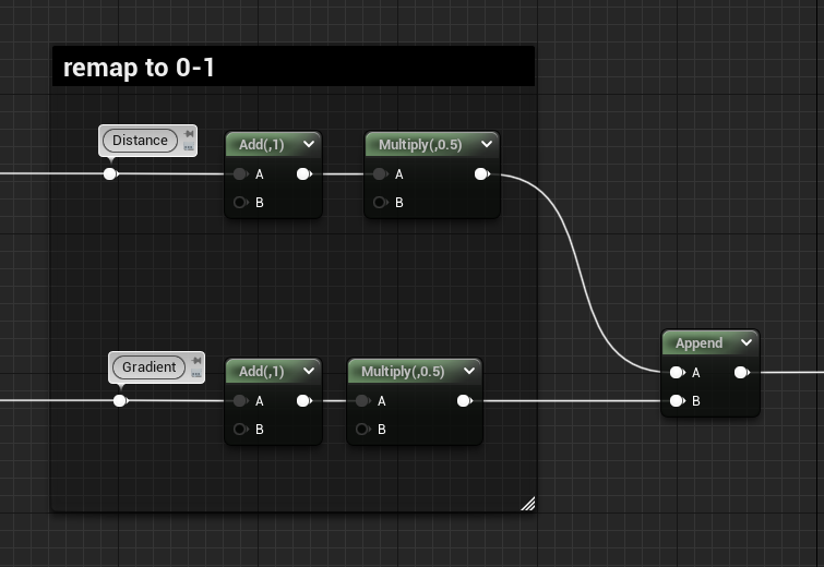
This is what it will look like:

Niagara

In Niagara you can use the built-in Sample Texture module, here you can feed your texture directly or have it as a user parameter, the only other thing needed is some UVs!
If you’re spawning the particles with the combination of “Spawn Particles in Grid” and “Grid Location” modules, you can use the attribute GridUVW that gets created. Otherwise, if you’re simply using a Shape Location module set to Box/Plane, like I’m doing, we need to make the UVs based on their position.

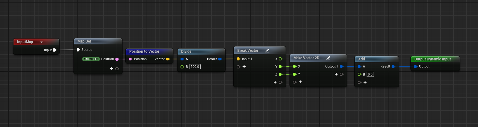
To do that I made a vector2D particle attribute called “UVs” and I’m setting it using the Scratch Dynamic Input. Below you can find the graph, I’m getting the position and dividing by the size of my plane (which is 100 in my case), then I’m making the Vector2D getting only the 2 axes I’m interested in and adding 0.5 to offset the origin from being in the center of the plane to a corner in the bottom.
Note that to make this setup work you need to have the Emitter be in Local Space, if that’s not possible you need to take into account the World Position of the Actor in the level and offset the particle position value accordingly (I believe you can do it by using the Engine Emitter Attribute “SimulationPosition”, but I’m not 100% sure).

Of course, if you need this setup in multiple Niagara Systems I suggest creating an actual Dynamic Input asset for it, with the size of the plane exposed as a parameter.

I might write something more in detail about this topic in a future post, for now, let’s get back to our SDF.

Now that we sorted out the UVs we can sample the texture with the Sample Texture module mentioned earlier, this module creates a particle attribute called SampledColor that contains the values of our packed texture. We can use a custom module to unpack it and remap these values back to -1 to 1 and create particle attributes for both the distance and the gradient.
This can be done by multiplying by 2 and subtracting 1, then since I want to make particles flow around the SDF shape I’ve rotated the gradient by 90 degrees and saved it as another attribute.
To rotate a 2D vector by 90 degrees you can invert the order of x and y and multiply x by -1:

(x, y) --> (y, -x)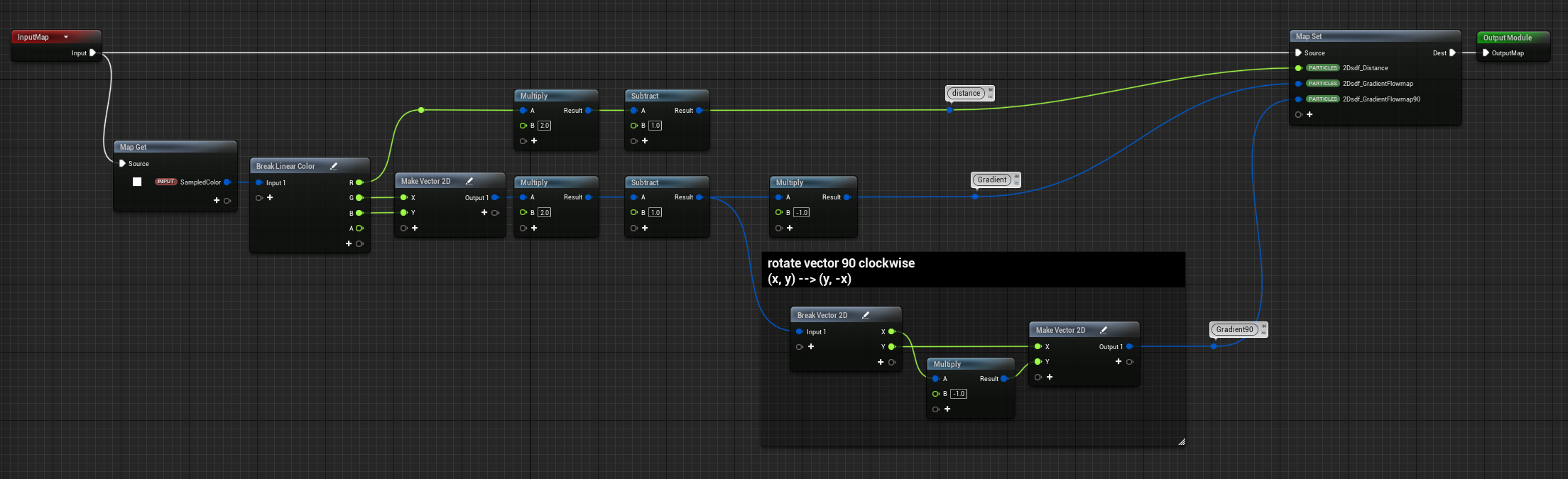

If we visualize the vectors of the rotated gradient they look like this:

Now if we align the direction of our particles using the gradient vector as is, we’ll get the result I showed during the explanation part of this post. What we can do is use the distance information as well to invert the direction base on if the particles are inside or outside the SDF shape:

We can use these vectors to attract the particles towards the shape’s edge, multiplying it by a force and adding it to the Transient Attribute PhysicsForce so that it gets applied to the velocity in the Solve Forces and Velocity module. We can do the same for the rotated gradient.

That’s the main logic needed to have particles move along the SDF edge:

The power of this setup is that if we can have the texture baked out if the SDF doesn’t move, but if it’s animated we can feed the RT directly and calculate the new SDF distance and gradient in real-time getting some very cool results like this one:

Anti Aliasing

Introduction

When working with these shapes and you’re using a Step function to visualize them, you might have noticed some aliasing or flickering around the edges, it’s not much since we are working with procedural shapes instead of using textures but in some cases, it might be more evident. Fortunately, there is an easy solution!

I did some research online on the topic and I would recommend you to read these 3 sources:

1. numb3r23 – Using fwidth for distance based anti-aliasing – the technique I used and will explain below 
2. mortoray – Antialiasing with a signed distance field – interesting read, but the SDFs, in this case, need to be calculated in pixels
3. drewcassidy – Antialiasing for SDF textures – might be useful if you’re working with SDF textures

Function

We can introduce some anti-aliasing using the Smooth Step function, we want the interpolation to only happen on the edge of the SDF shape, basically the size of one pixel. To achieve this we need to calculate the “anti-aliasing-factor”, which will basically tell us the rate of change in the distance field.
This can be calculated by feeding the distance of the SDF directly in the fwidth function: 

float aaf = fwidth(dst);

Unreal’s Material Graph doesn’t have a node for that, but fwidth is simply the sum of the absolute values of ddx and ddy – check out this video to learn more about these three functions.

dx = ddx(v);

dy = ddy(v);

fwidth(abs(dx) + abs(dy));

Now, the size of the rate of change in the distance field given us by the “anti-aliasing-factor”, determines how wide the Smooth Step interpolation needs to be in order to fade the edge of the SDF shape:

return 1.0 - smoothstep(radius - aaf, radius, dst)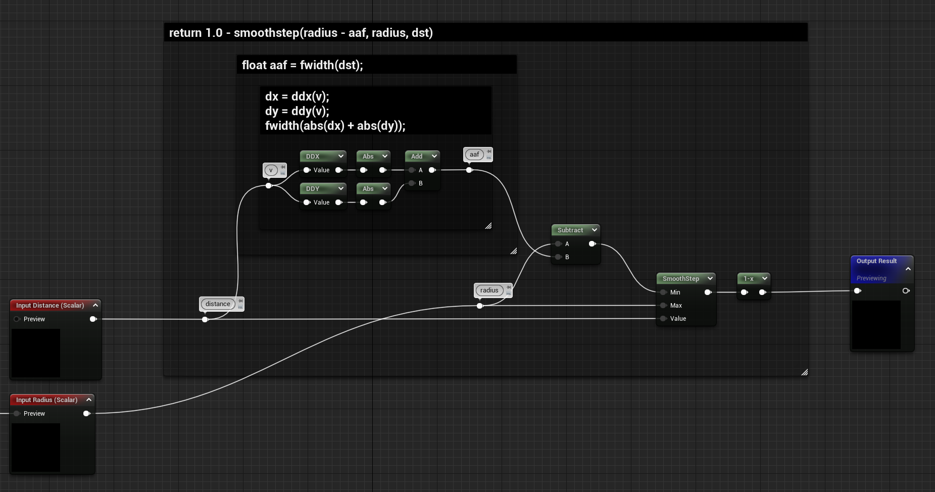

I would replace the step function with this one almost in every scenario, it’s very useful when using the SDF as the opacity for a masked material or the alpha when lerping between two colours.

Conclusion

For now, this is everything I wanted to share about 2D SDF, in the future I would like to experiment more with 3D SDFs to create some interesting FXs with Niagara.
I hope you found this post insightful, have a good rest of the day!