Introduction

This is the third part of a series of posts about 2D SDF, check out the first one where I show some simple shapes and explain the basics to visualize them, and the second one where I show different ways to combine them!
I think it’s very useful and valuable knowledge for every Technical or Environment Artist, but really for anyone that works with materials.
In this post, I will cover ways to manipulate the space used to sample these shapes, as well as share some extra tips I’ve learned along the way.
As I mentioned before, everything I will cover is not new knowledge, I’ve learned it all by reading Ronja and Inigo Quilez’s articles which I highly recommend for getting a better understanding.
The focus of my posts is to show how their content can be recreated in Unreal Engine and its Material Graph.

I’m sorry again if this is another long post, but I hope it’s worth reading, enjoy!!

Distortion

I found a couple of ways to add some distortion to the perimeter of the shapes.
The first one involves sine waves, while the second one 2D or 3D noises. The only thing to flag is that doing this will make the distances of the sdf functions less precise, but if the intensity and the amount of these distortions are low, in most cases this is not a problem.
For all the direction examples shown below, I’m going to use a simple square shape.

Wobble

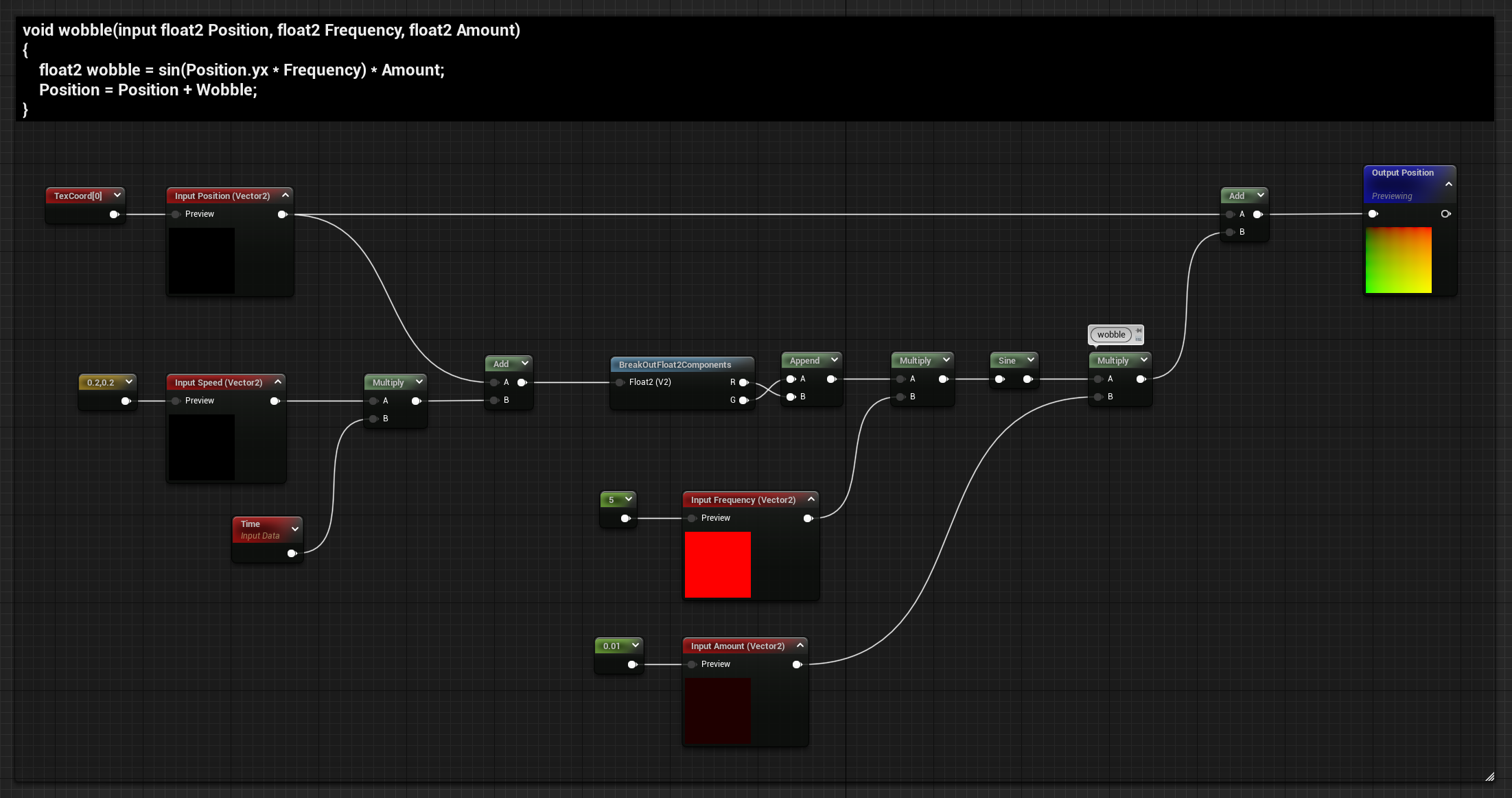
Distortion can be added using sine waves, we can do this by calculating two different sine waves, one for each axis, and adding it to the position used to sample the sdf shape. All the inputs expect a vector2, this is so that you can have separate control on the two axes.
To calculate the wobble we need to flip the x and y components, then it can be multiplied to control the frequency, feed the result to a sine node and multiply it again to control the intensity. The distortion can be animated by adding time before flipping the position, and the speed can be controlled with another multiplication.

void wobble(input float2 Position, float2 Frequency, float2 Amount)
{
    float2 wobble = sin(Position.yx * Frequency) * Amount;
    Position = Position + Wobble;
}

Multiple wobble functions can be added together to get more variation and a more complex result

Noise

For the noise, the logic it’s the same, do some multiplications to control its intensity and speed and then add it to the position before sampling the sdf shape.
Compared to the wobble, I noticed that with this method you might get even more imprecise results and artifacts on the perimeter of the shape, so be careful with it.

You can use a 2d or 3d texture based on your options, I prefer using a 3d noise because this way I can animate it through the depth axis and easily get it to look like it’s morphing.
In the example below I’ve used the built-in procedural noise node, I’ve just reduced the number of levels to 3, and its scale.
I didn’t create a function for this since you might need a different one for each type of noise setup you are going for, however you should definitely make one if you’re using the same setup multiple times.

Extra

Now, I want to point out that you should definitely play around and experiment. For example, I asked myself what would happen if I did similar operations after sampling the sdf shape instead of manipulating the position.
Well, you get slightly different results of course, but is that the correct way of doing it? Who cares, if you like the result it doesn’t matter. Tech Art is not always about knowing and correctly applying techniques and math, in the end, our aim is to get some beautiful results. You don’t always need to understand the logic behind it, sometimes it’s fun to just chuck together some nodes and values to see what comes out, you never know what you are going to get!

Below you can find some examples of some experiments, with both sine waves and noises.

Sine Waves:

Comparison of adding or subtracting noise:

Two similar setups where the noise is combined in a way so that it only removes information or inflates the shape:

Mirroring Options

Like in the way we do the shape’s deformation we can manipulate the position to get some other results. Below I’ll show some useful mirroring options.
Relying on manipulating the space and getting mirrored results it’s a lot cheaper than sampling shapes multiple times, this way you can achieve some quite complex but cheap effects.
For all the mirroring options examples shown below, I’m going to use always the same sdf combination of a triangle and a circle, they both have a slight offset from the center, added using the basic transformation functions shown in the first post I made about sdfs.

Mirror

Simple Mirror

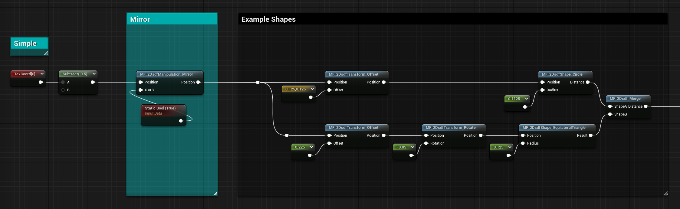
Doing a basic mirror it’s very simple, we can just get the absolute values of one of the two axes:

void mirror(input float2 Position)
{
    Position.x = abs(Position.x);
}

For the function, I’ve also added a Static Switch to flip between mirroring on the X or on the Y axis.

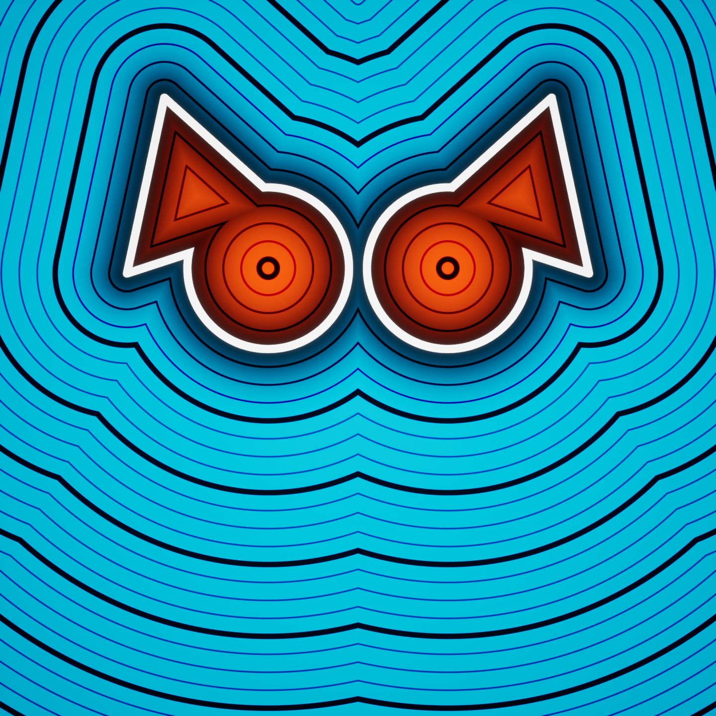
Rotate Mirror

You can combine this with some basic transformation functions showcased here, I’ll show you some tests with the rotation.
If you add a Rotate function before and after the Mirroring one, and you multiply by -1 the Rotation input for the second Rotate function, you can isolate the rotation to the Mirror axis:

Rotate only Shapes

Adding the Rotation function only after the Mirror one keeps the axis stationary and only rotates the position resulting in an interesting effect:

Rotate Everything

On the contrary, putting the Rotation function before the Mirror makes both the axis and shapes rotate:

Normal Cells

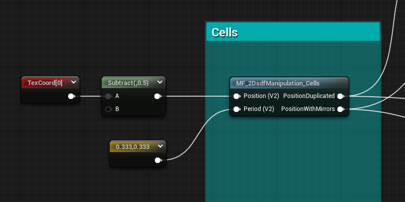
We can also tile the position in a way so that it creates cells, this function gives 2 different outputs, the first one duplicates the position like a classic tiling you can find working with textures, while the second one it’s also mirroring the position.
The problem with the first output is that if the shape overlaps the edge of the cells it creates some artifacts, which doesn’t happen with the mirroring option, something to keep in mind.

They both use some fmod trickery, the duplicated position function is:

void cells(inout float2 Position, float2 Period)
{
    newPosition = fmod(Position, Period);
            //negative positions lead to negative modulo
    newPosition  += Period;
            //negative positions now have correct cell coordinates, positive input positions too high
   newPosition  = fmod(Position, Period);
            //second mod doesn't change values between 0 and period, but brings down values that are above period.
}

For the Mirror output, we need to calculate the Cell Index to know which cells need to be flipped, we can add this to the previous code:

float2 CellIndex = floor(Position / Period)
float2 flip = abs(fmod(CellIndex, 2));
Position = lerp(newPosition , period - newPosition , flip);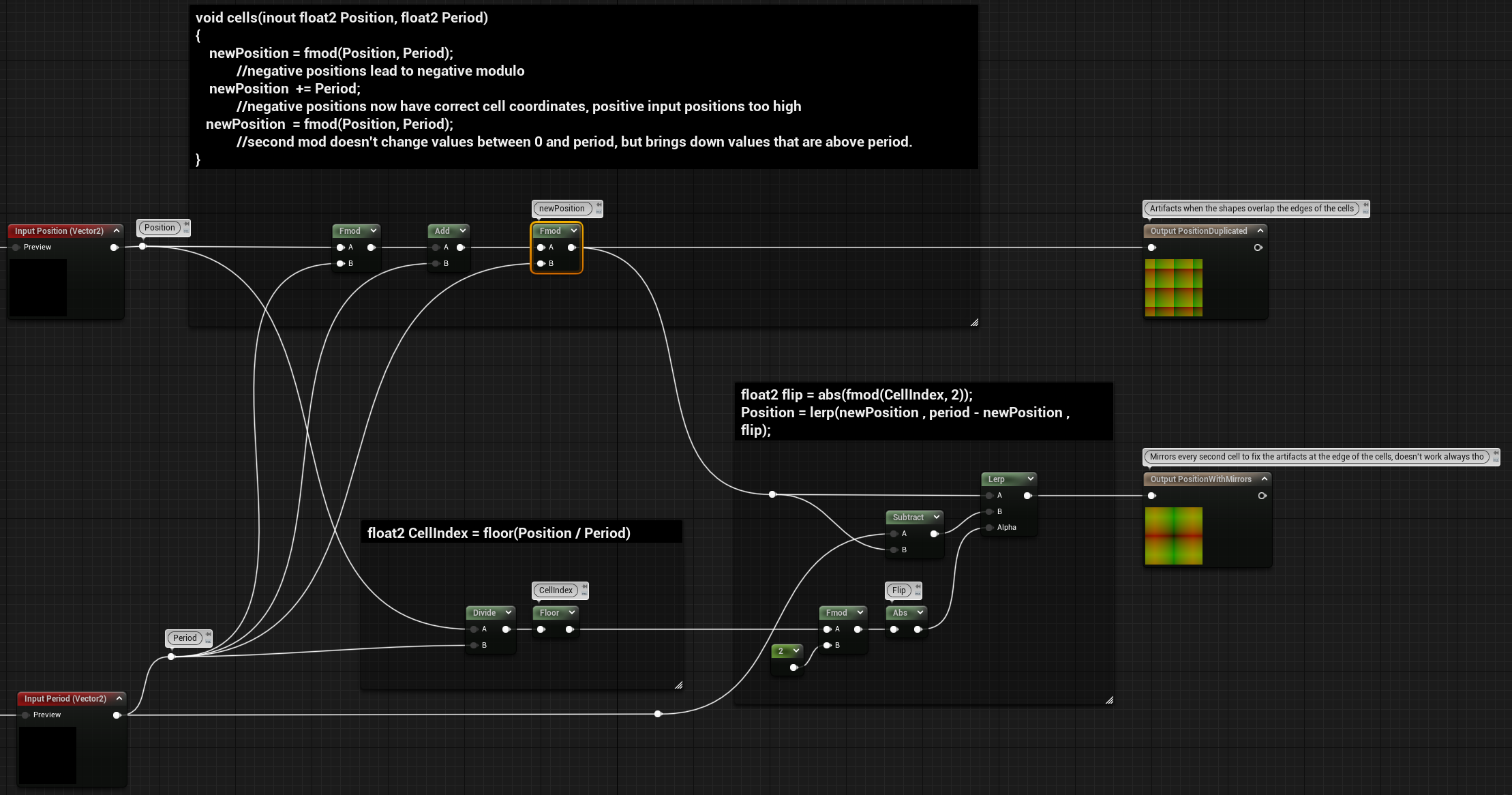

Here’s the comparison of the two outputs, duplicated position on the left and mirrored version on the right:

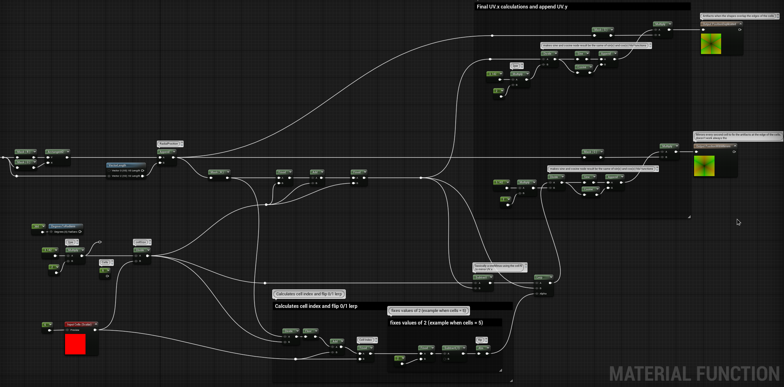
Radial Cells

This one is a little bit more complex, as it always is when rotations are involved, as I mentioned before check out Ronja’s tutorial for a more in-depth explanation of how this works.
Regarding how to recreate it as an Unreal Function, like before, the function has two outputs, one for the duplicated position and the other one with the version with mirrors.

I need to mention that I’ve run into some complications when using Unreal’s Sine and Cosine built-in nodes, I mentioned it in one of my previous posts as well. I realized that the input they take is normalized, so that when you feed a 0-1 value it outputs one wavelength. This makes these nodes a lot more useful and intuitive when using UV coordinates as inputs. However, the hlsl sin() and cos() functions to output one wavelength need 2pie as the input:

So, for the calculations we need in our function we need everything in radiants, so the hlsl function would give us the expected result.
However, you can find on Unreal’s Documentation that using custom nodes “prevents constant folding and may use significantly more instructions than tan equivalent version done with built nodes”, so for something simple like this I would try to avoid the custom node and instead try to get the same result using the built-in nodes.
In conclusion, this entire explanation was just to say that we need to divide by 2pie the inputs that go into our sine and cosine nodes, to recreate the same result of the hlsl functions.

The function is:

float radial_cells(input float2 Position, float Cells)
{
    const float PI = 3.14159;
    float cellSize = PI * 2 / cells;
    float2 radialPosition = float2(atan2(Position.x, Position.y), length(position));
    float cellIndex = fmod(floor(radialPosition.x / cellSize) + Cells, Cells);
    radialPosition.x = fmod(fmod(radialPosition.x, cellSize) + cellSize, cellSize);
    // Add this to make the version with mirrors
        // float flip = fmod(cellIndex, 2);
        // flip = abs(flip-1);
        // radialPosition.x = lerp(cellSize - radialPosition.x, radialPosition.x, flip);
    sincos(radialPosition.x, Position.x, Position.y);
    Position = Position * radialPosition.y;
    return cellIndex;
}

And here’s the graph, where the sine and cosine inputs are divided by 2pie:

Here’s the comparison of the two outputs, duplicated position on the left and mirrored version on the right:

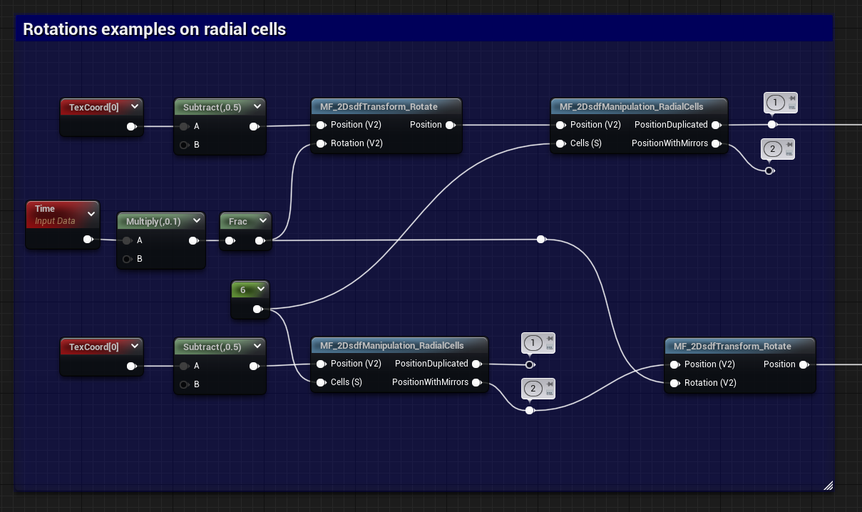
Rotation Examples

Like before, we can add some fun rotations and get different results based on if we do the radial mirroring of the UVs before or after the Rotate function.
For the sdf shape in these examples I’ve only used a triangle, with some offset to move the shape in the visible UV space:

The graph:

And here are the results,
rotation added before the mirroring:

Rotation added after the mirroring:

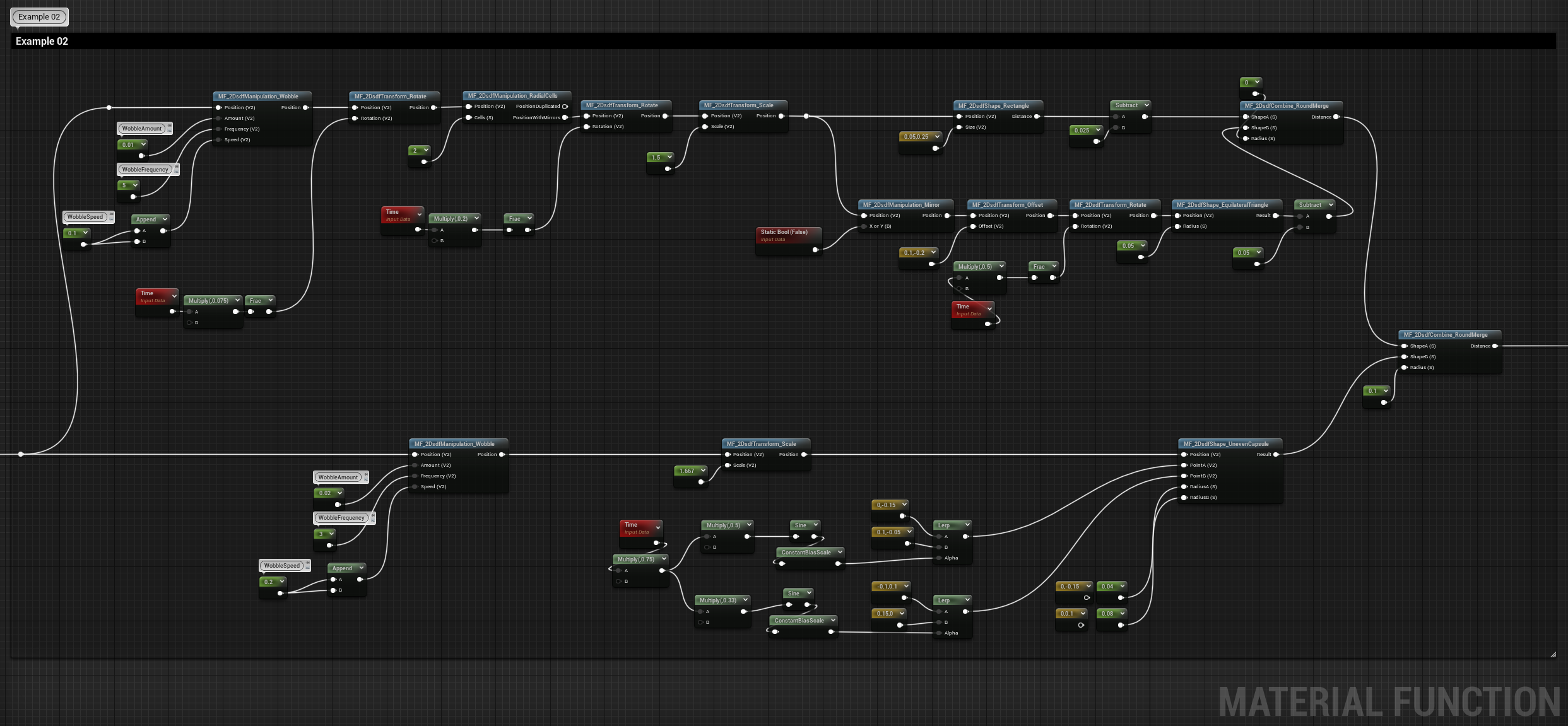
Library Examples

Here you can find a couple of examples of how to use together the sdf functions I’ve shown in these past 3 blog posts, to create some random morphing shapes.

For the first example, there are a couple of shapes floating around with their position animated and then merged together.

While this second one also has some shapes with their position animated, I’ve also added a mirror function to get a more complex result.

Conclusion

The next post will probably be the last one about this topic, I’ll show how to make a flow map using a Sign Distance Field, which can then be used in the material to warp a texture or in Niagara to drive the location of particles. I’ll also mention something about Anti Aliasing.
I hope you found this post useful, have a great rest of the day!