Introduction
In this post, I would like to outline a technique I frequently use to debug the look of a gradient, as well as trying to take it further by exposing some extra controls to increase its usefulness.
I’ve been inspired, for a while now, to try and recreate, within Unreal’s Material Graph, something similar to Substance Designer’s Cross Section node.
By doing so, I ended up finding a couple of rabbit holes that I hope I’ve been able to explore only deep enough to get what I was looking for without wasting too much time!
I’ve structured this post more like a broad guide/tutorial to showcase various techniques, but the structure very much follows the order of things I’ve tried during my exploration.
I hope it makes for a fun read!
Cross Section Sampling
Simple Gradient Visualizer
I’ve already shown this technique in another post I made a little while back. If you want to know more about it, check it out here: Gradient Visualizer Material Function
It can be used to visualise any type of one-dimensional horizontal gradient.
For example, if you have a gradient that is placed along the U axis of the UVs, you can add it to the V axis and floor it, or subtract it and apply a ceiling operation. Both options will result in displaying the target gradient.


This technique is very useful to exactly visualize the values of the 1D gradient.
Below, I’ve applied the same logic to one of the channels of a colour curve added to a curve atlas. The linear U gradient is plugged into the CurveTime input of the node, then I’m doing the same adding and flooring operations with the linear V gradient. The result is exactly the same as the curve’s profile set in the curve asset.


Noise Texture
The same logic can be applied when sampling a texture; the linear U gradient that was used as the CurveTime input earlier is now appended to a “CrossSection” float parameter to create a 2D vector used to sample the texture. The float parameter defines at which point of the V axis the texture gets sampled, resulting in a 1 dimensional gradient output.
Below, you can see this logic applied to a Perlin Noise texture, using a Cross Section value of 0.5, which samples a horizontal slice in the middle of the texture.

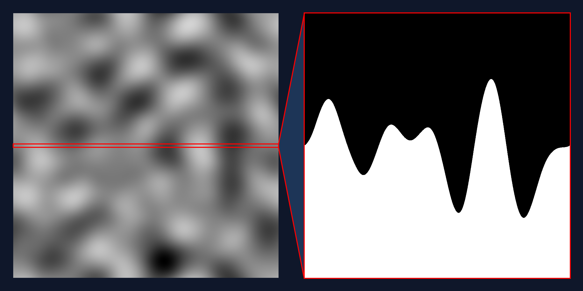
Sample V
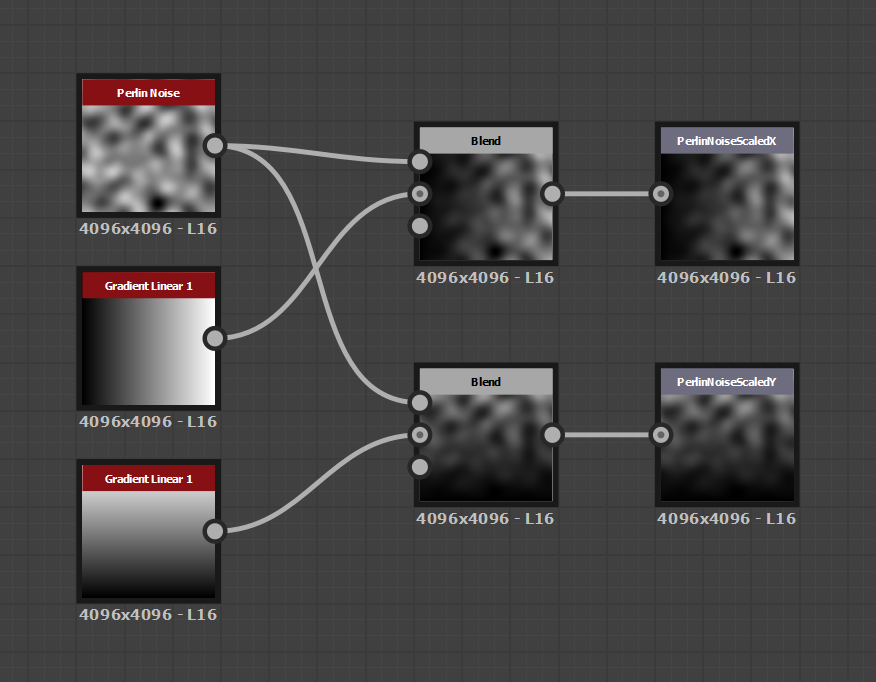
At the moment, the setup it’s only sampling the U axis of the texture, but control can be exposed to sample the V axis instead, just by introducing a swizzle operation on the UVs before the texture is sampled.
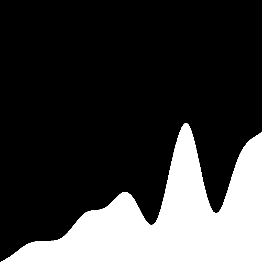
To debug this, I’ve made 2 textures with a linear gradient baked into them, one for each axis. This helps display which axis is currently getting sampled.
In the images below, I’m sampling over the U axis, using the texture with a U linear gradient applied.

In these other images, I’m sampling over the U axis, using the texture with a U linear gradient applied.
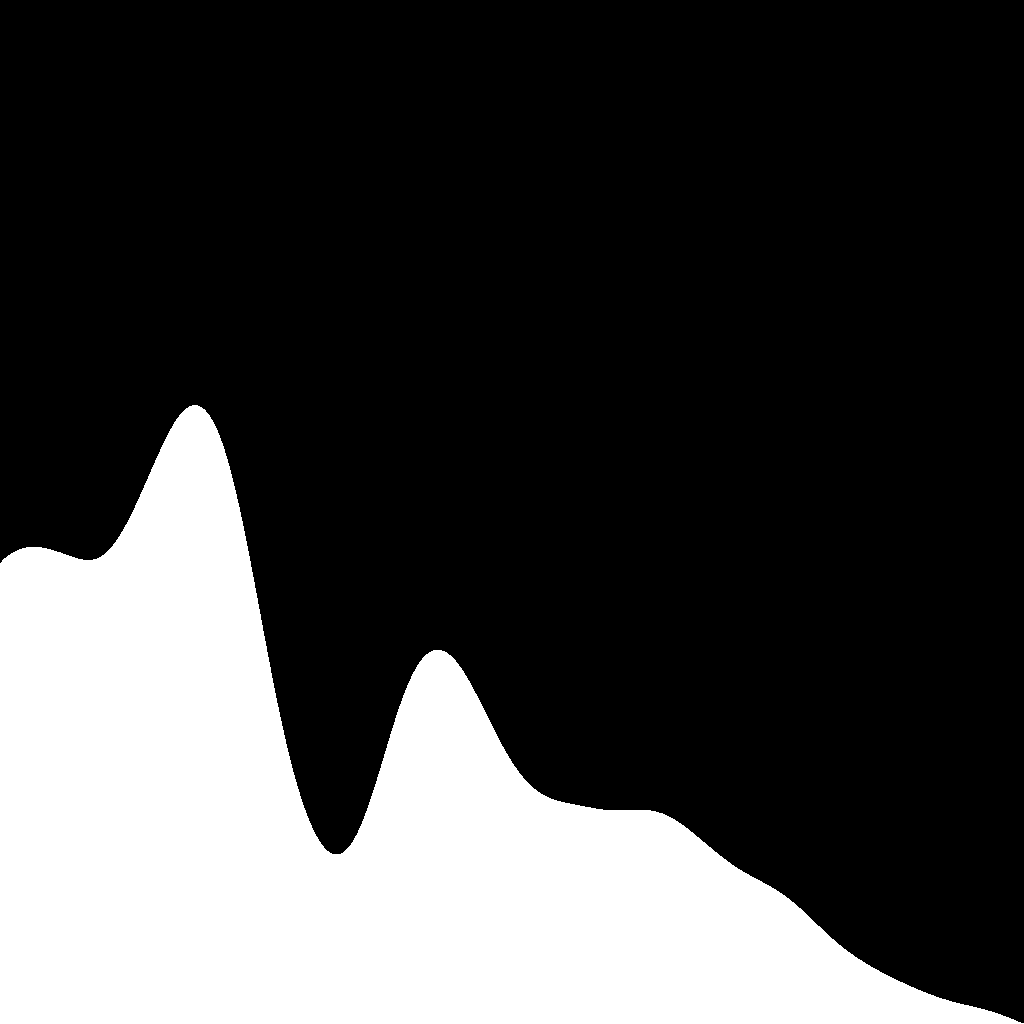

Looking at the result of sampling the U axis, I initially thought it should be mirrored to be more visually intuitive. However, when using the cross-section node in Substance Designer, the output is the same as the one above.
It really depends on what the UVs or your preview mesh look like, in Unreal, the V axis of the material graph’s default plane starts with 0 at the top and becomes 1 at the bottom. I believe this is because frames are generated from top to bottom, and monitors also refresh from top to bottom.
You can add a one minus node if you want to change its orientation; however, I’ve just left it as is to keep the graph simpler.
Vertical Output
Similarly, you can also change the axis in which the output is displayed by adding a couple of switches, one before the texture gets sampled, and one after it.
The graph below shows the vertical output in action, using the texture noise with the V axis scaled.


Artifacts
Quality and Texture Compression
If you zoom in and noticed that there is some jitteriness on the curve, it’s probably because you are using a 8bit texture instead of 16bit. I’ll try not to go too much into details in this post and maybe explore the topic further on a separate post (but I don’t know if I’ll be able to contain myself). It’s probably because the texture you are using was saved as a TARGA.
It might not be clear with only a glance, especially on noises, but if you zoom in, you can see the 16-bit version is a lot smoother:

Here’s a closeup:
If unaware of this 16 and 8-bit difference, you might be tempted to try and increase the resolution size of the texture, which might help when looking at it at specific distances, but the jitteriness it’s still there when zooming in.
Here’s a comparison of using a 1k vs a 4k texture:
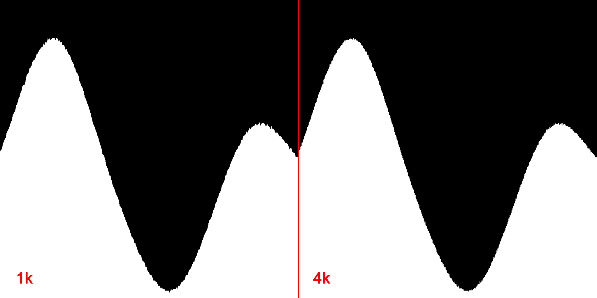
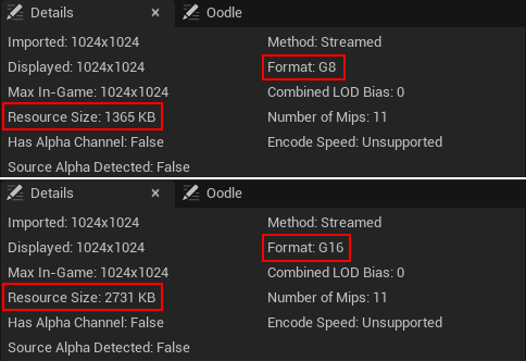
That’s because there is a limit in how many greyscale values a 8bit texture can contain. A greyscale 8bit texture can contain 256 shades of grey, while a 16 bit can contain over 65000. However, the resource size also increases. In the case of the Perlin noise 1k texture I’m using for this little project, it doubles, with the compression settings set to Greyscale, it goes from 1365KB to 2731 KB.
It’s not entirely true saying that this jitteriness it’s solely caused by the texture being 8bit, the compression settings and the filtering options used are also contributing to this. For example, if you set the filtering to “Nearest”, you can see more closely what value each pixel has stored, resulting in a pixelated look.

If you don’t need that much detail in the gradient, want to use a 8bit texture, but still want to get rid of the jitteriness, you could sample lower Mip Levels since they get generated using some filtering that smooths the results. This reduces jitteriness, but the curvature will look more segmented.


However, it doesn’t matter what you do to the texture; if it’s 8-bit, it will never result in a completely smooth look.
For that, you’ll need to use a 16-bit one, and to try and keep the memory footprint in check, you can play around with different compression settings and resolution sizes.
Non-Tiling Texture Artifact
When using a non tiling texture, there is an artifact showing up where the texture repeats. These artifacts appeared when I started using a texture that has the gradient scaled on one of the axes.
In the image below, you can see it on the left side of the texture.
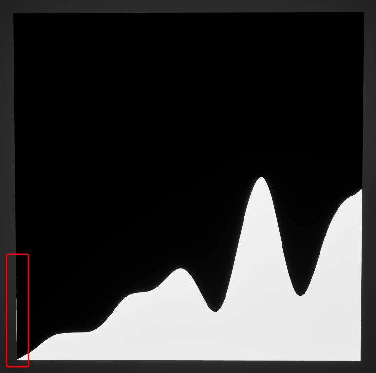
This is caused by the filtering operation applied to the texture. The engine assumes the texture is tiling, so when the filtering processes the pixels placed on the edges of the texture, it will consider the pixel on the opposite side as their neighbours.
This behaviour appears by default for any texture you import. When importing tiling noises, this is the desired result, but it’s not for texture sets made for assets. In the latter case, tho, usually the UV shells have padding that prevents them to touch the edges, preventing this artifact to appear.
However, it’s something to consider since it might be relevant when mipmaps are generated, lower resolution textures could cause these values to spill into the UVs of the asset, since the padding won’t be enough any more to prevent it.
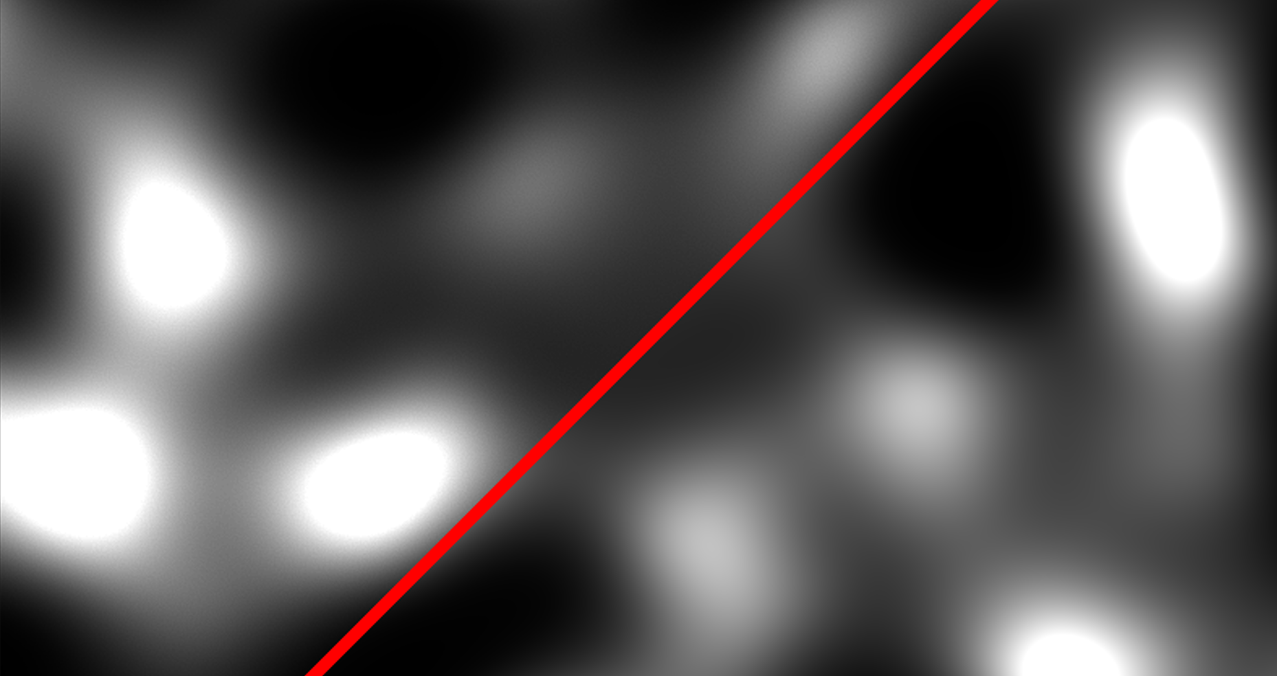
Here’s a random example using the engine texture called “DefaultCalibrationColor”; you can see on the right side of the texture there is a white vertical line, which is caused by the white pixels on the other side of the texture.
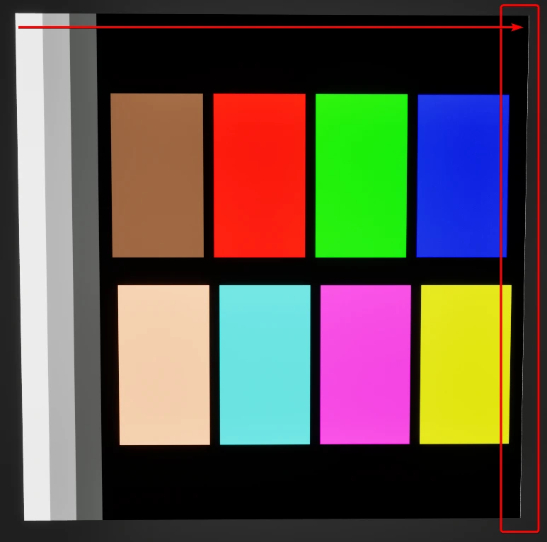
To address this, the filtering option can be “removed”, setting it from its default value to “Nearest”; this option does not take into consideration neighbour pixels, removing the artifact. However, this is usually not the desired way to fix this issue.
Instead, on most occasions, it might be better changing the tiling method of the asset, from “Wrap” to “Clamp”.

Or, if you know what you are doing, you can edit the texture sampler in the material, setting the Sampler Source option to “Shared: Clamped”.

(The Shared option creates a new, unique atlas texture that contains all the textures used in that material. This is a useful workflow when working on landscapes, since usually a lot of textures are required for it, more than the allowed limit of 16, doing this reduces the amount of texture sampled since they get all combined into 1, preventing the limit to be reached. However, for example, this is not a great option when making FXs, because FX textures are reused multiple times in different materials across the entire project. Setting the sampler to “Shared” means that the texture gets essentially loaded into memory multiple times, because it gets included in a lot of different unique atlases).
Going back to this cross-section exploration, I’m this example, I wouldn’t use a non tiling texture at all; the ones I made were just for debugging purposes, to visualize which axis was getting sampled.
If I needed to scale the noise, I would instead keep using the tiling texture and apply the linear gradient after the texture gets sampled, scaling the result before visualizing it.
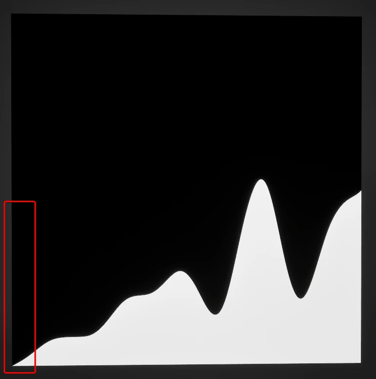

Pseudo SDF Gradient
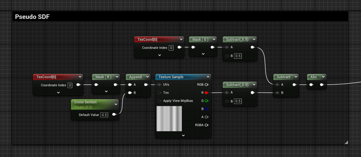
There is a little trick that can be applied, which allows one to achieve a gradient similar to an SDF.
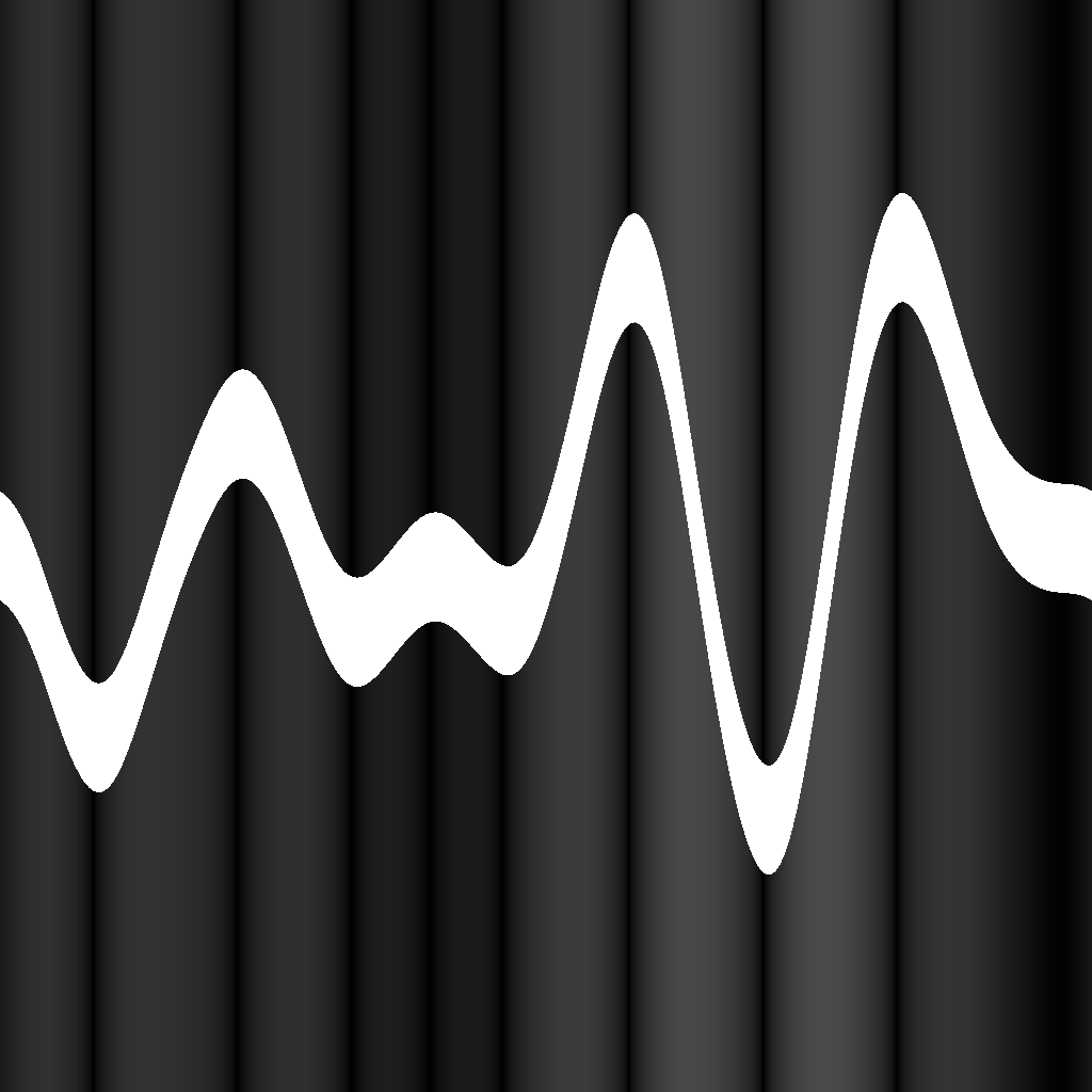
This can be done by subtracting the sampled values from the linear gradient of the axis in which the visualisation happens, but before doing this subtraction, both gradients need to be 0 centred by subtracting a value of 0.5 from both of them. Then, with an absolute operation, negative values can be converted to positive. If you then treat this gradient as if it were an SDF, and apply a Smooth Step and One Minus operation to it, you can visualize the curve as a line with thickness.
However, it’s not really an SDF because the gradient doesn’t fully represent the distance from the curve; it only does it considering one of the 2 axes.
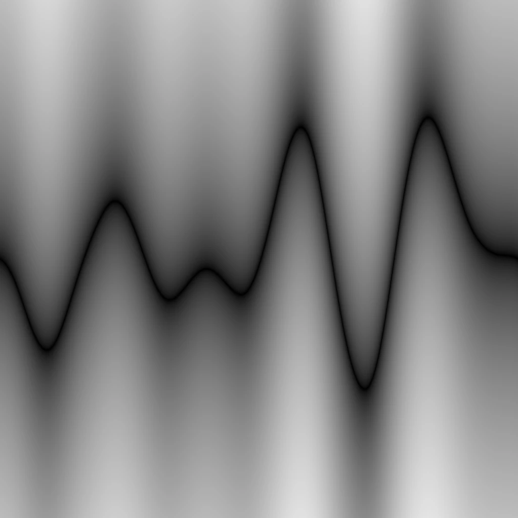
The fact that this is not an SDF becomes clear when the thickness of the shape is increased. The result is not uniform; the gradient is thinner when the curve is going up or down, and it’s thicker when it’s going horizontally.

Derivative Compensation
From Wikipedia, the definition of derivative is:
>"[...] a fundamental tool that quantifies the sensitivity to change of a function's output with respect to its input. [...], is the slope of the tangent line to the graph of the function at that point. [...] often described as the instantaneous rate of change [...]".
It’s the rate of change of a function at a specific point, representing the slope of the tangent line going through it.
I thought I could compensate for this thickening behaviour by calculating the curvature’s rate of change, and thickening the line when the rate is higher.
The rate of change can be calculated by sampling the texture a second time using a small step offset increment, subtracting it to the original sampled value, negative and positive values will represent if the slope is ascending or descending. In my case, I only need the information of “is changing”, so I applied an absolute operation to transform the negative values to positive. The bigger the stepping offset you apply, the greater the rate of change sampled will be, but it will also be less precise, since it will compare two points that are further apart from each other.

I tried applying this derivative to the gradient in various different ways, but I always get an additional “kink” when the divergence gets near to 0.
Graphs Attempts:
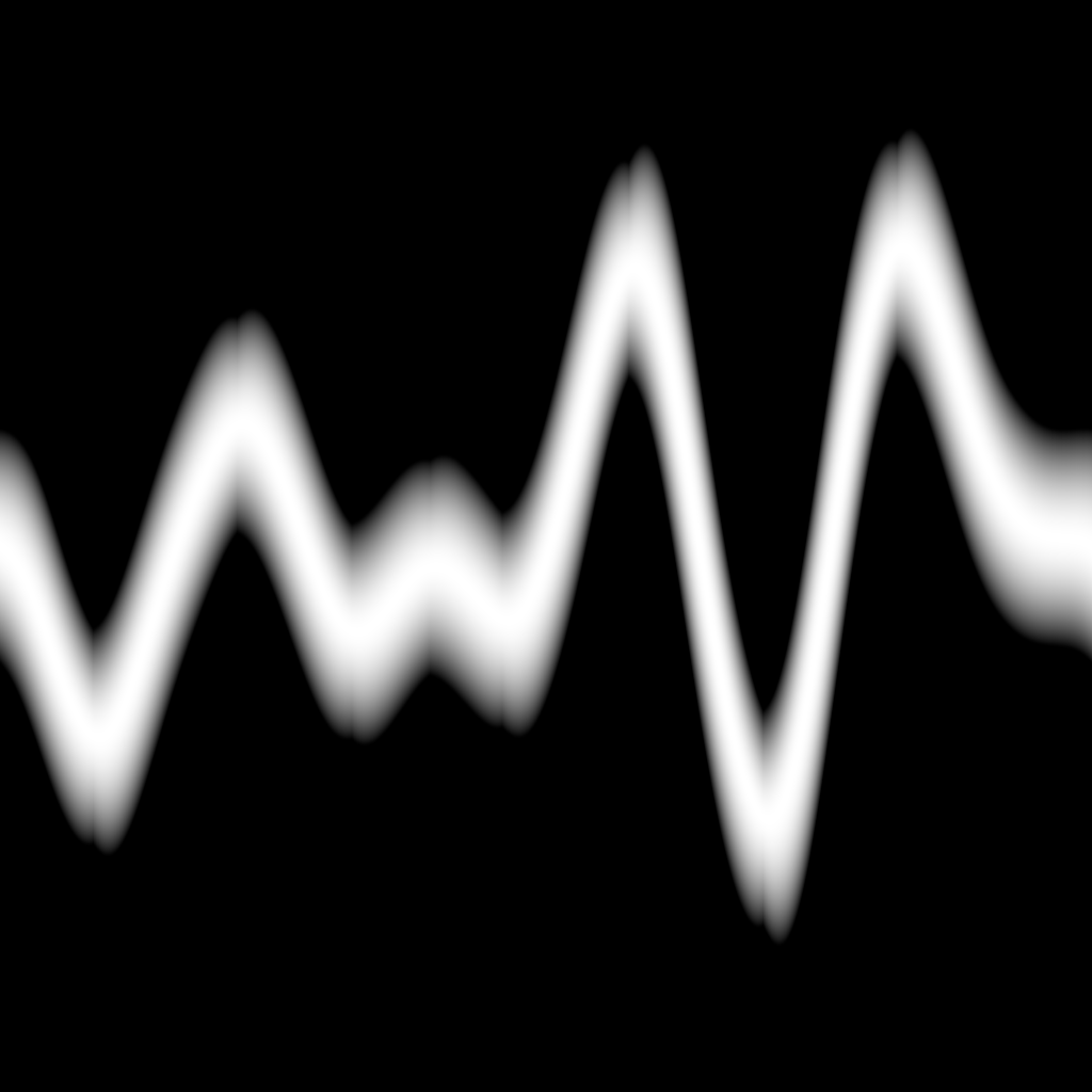
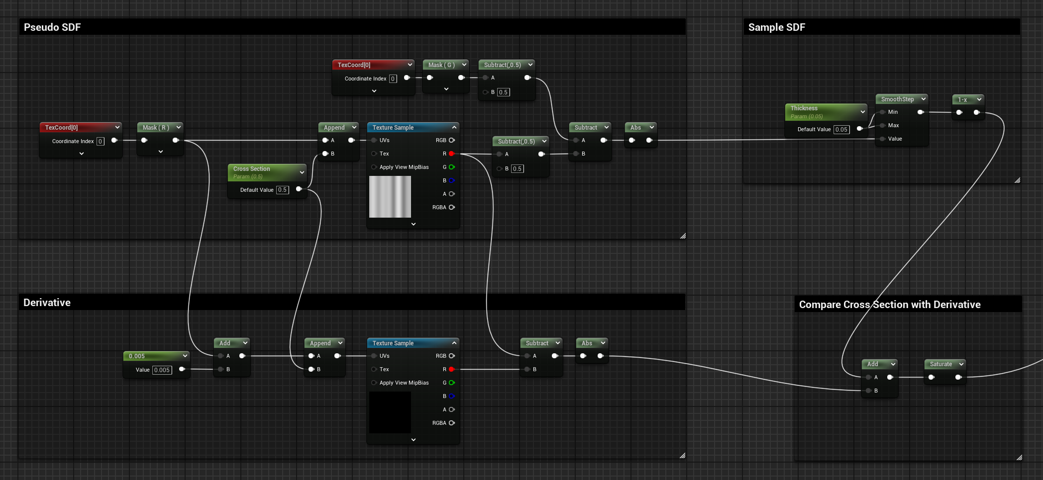


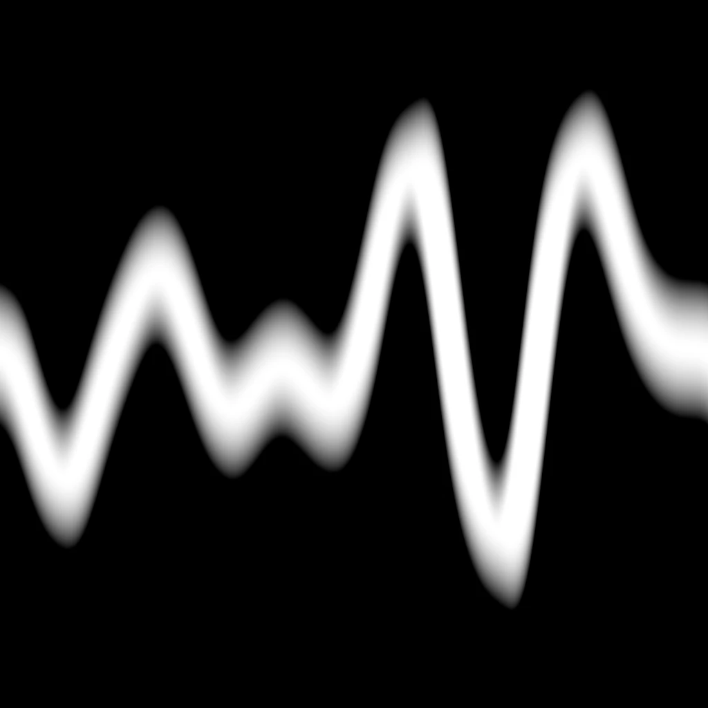
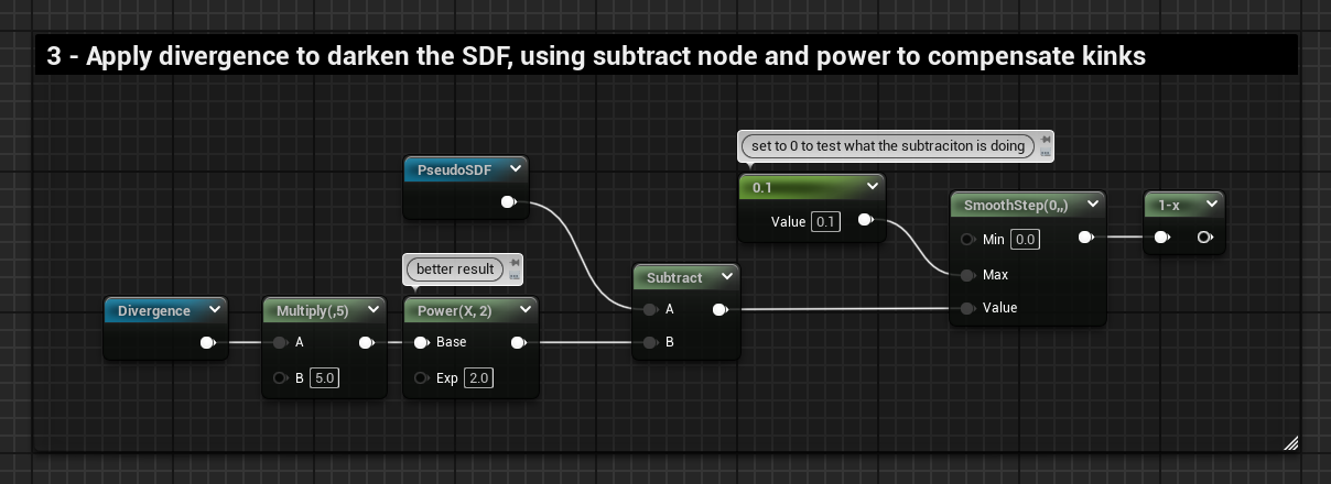
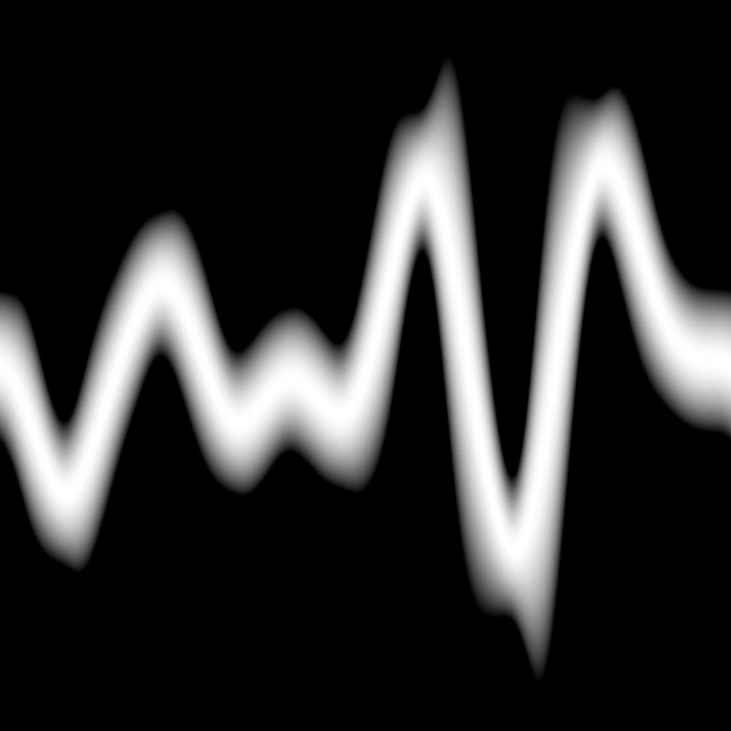
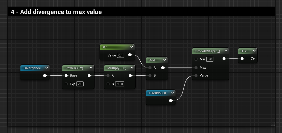
The 3rd attempt is the best result I could get, but the thickness is still not uniform, and if I play around with the values to improve it, the kings also get scaled up. Moreover, the gradient is also skewed.

Here you can see how the divergence is contributing to the final result:
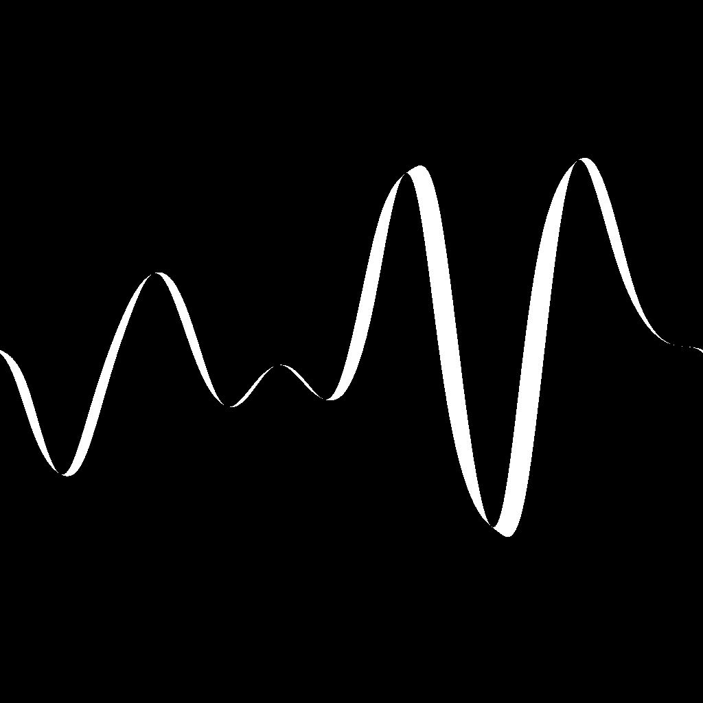
After these failed attempts, I checked the Substance Designer node and noticed that when the “Drawing style” is set to “Gradient mirrored”, the result also suffers from this thickening issue, suggesting that they are applying the same or very similar operations.
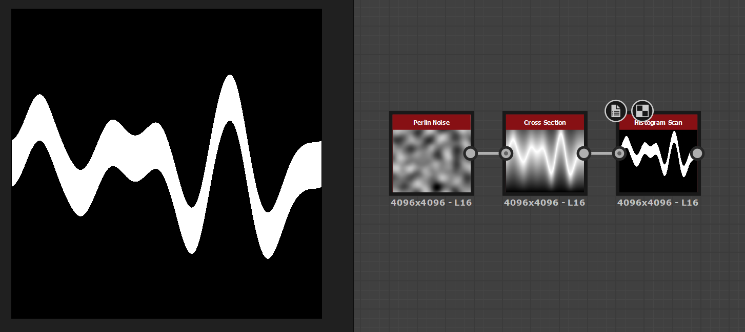
However, there is one setting, which is the “Line” Drawing Style, that renders the line with a perfect desires thickness.
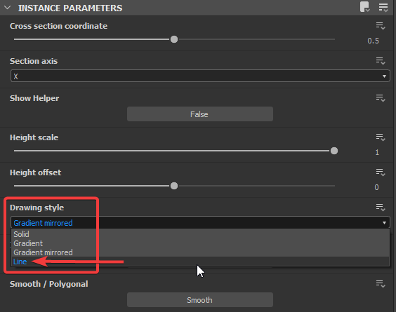
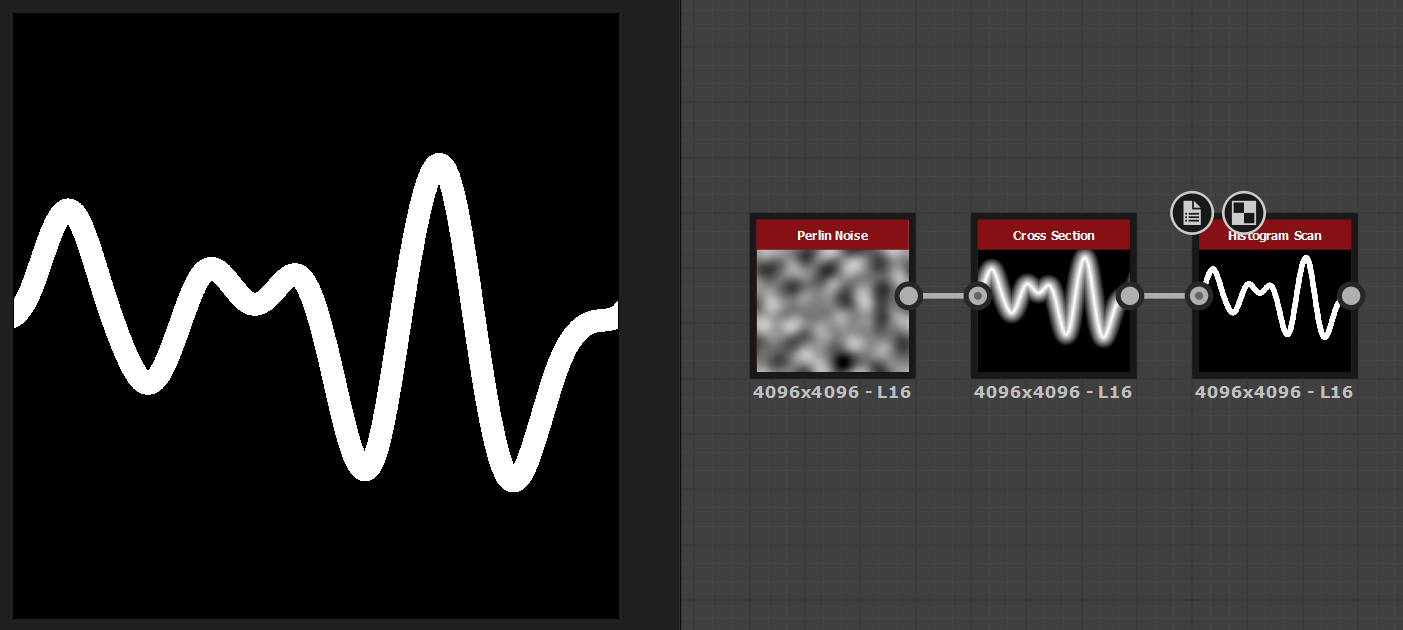
This is because the Line style is iterating over the gradient using an FX-Map node, and generating a lot of little segments based on the user defined parameter “Segment amount”, which are then combined together, giving the illusion of one smooth curved line.
SDF Segments
Substance Designer Node Breakdown
Let’s investigate the Cross Section node in Substance Designer, specifically its “Line Drawing Style”.
If you search for the node in the Library and right click it you can find where the sbs file for the node is stored, all the nodes that are available for you to use have been created within the software, and can be opened for inspection (excluding only nodes that are in the categories “Atomic”, “FxMap” and “Functions”).

The cross_section.sbs file contains 2 graphs:
- cross_section → where the main logic is
- spline_render_position → specifically to generate the “Line” drawing style
I’ve explored both graphs and added some comments to roughly describe what each node is doing. I’ve also added some additional nodes to debug the values. This is what they look like:

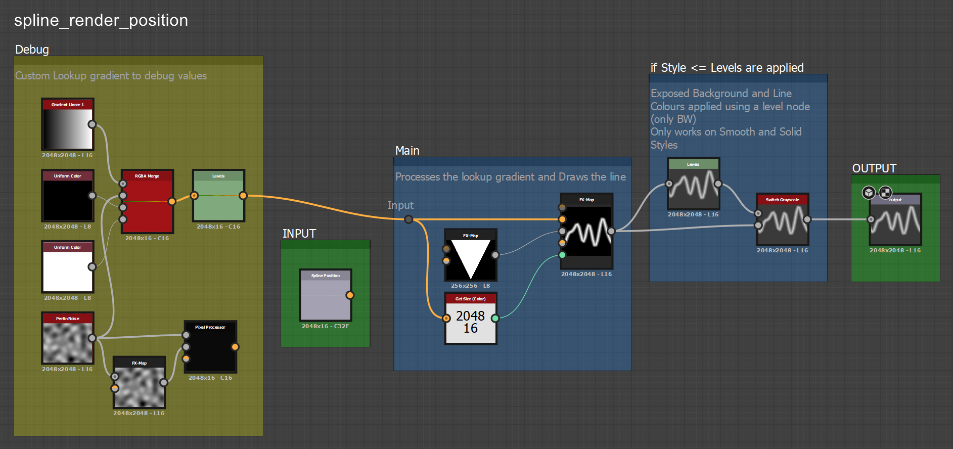
Feel free to explore the graph by yourself. What I wanted to bring attention to is how the Draw Style “Line” is generated, which is through a
FX-Map node inside the spline_render_position graph.
I haven’t used the FX-Map node much, so my definition might be incorrect or imprecise, but from my understanding, it’s a powerful node that allows you to iterate multiple times over some defined logic, with the help of “Iterate” and “Quadrant” nodes, which are customizable with your own functions. The iterate node defines how many times the logic runs, while the quadrant node defines the operation that gets applied to the pixels.
The nodes contained in the FX-Map node have properties that can be constrained to custom functions; this is what the one used in the cross-section SBS file looks like:
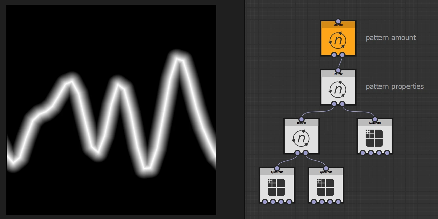
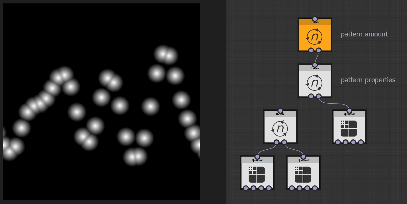
Feel free to explore the various functions setup in these nodes, to make your life easier, you can first find out what kind of logic is contained in each node just by unplugging some of the quadrants, isolating the logic of each of them.
Below, you can see the quadrant on the right isolated. It’s interesting to note that all these points are placed equidistant from each other when observing only the U axis; it’s only the distance on the V axis that is not uniform. This is because for all these points, their U axis position is defined by the iteration count, while the V comes from the sampled noise at that location.
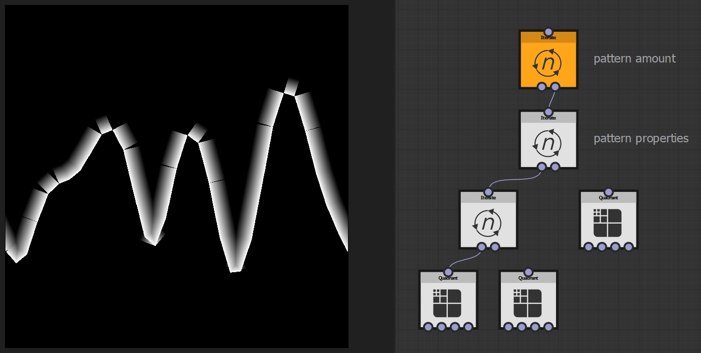
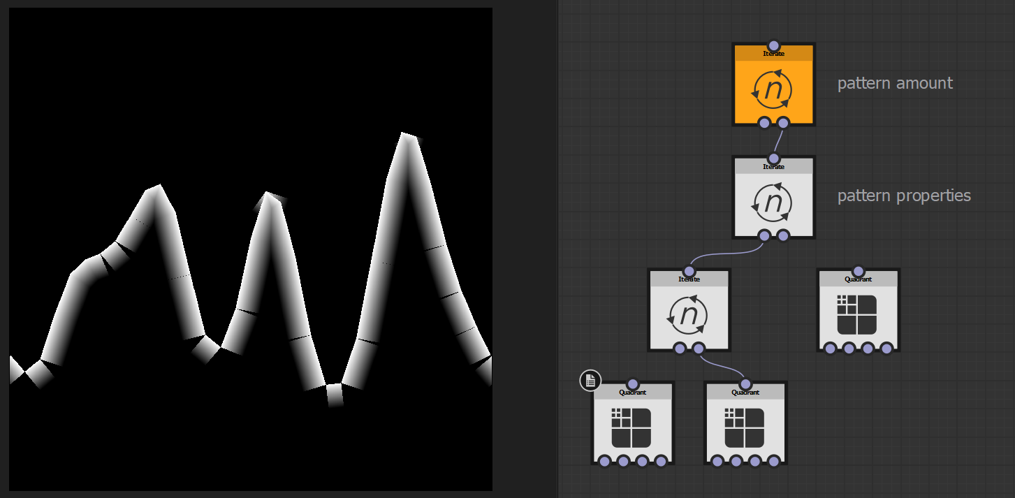
Here’s the quadrants on the left isolated, the logic is stamping little a lot of short gradients between the defined sampled position, using the correct orientation. The segments’ length changes based on the difference in the sampled value, between the head and tail, creating segments of various lengths.

Also interesting to note is that the segments are, in turn, split into two, with the upper and lower gradients drawn separately:
Within Unreal’s Material, we can recreate a similar setup, but instead of “stamping” a sphere and linear gradient segments, we could calculate a Sign Distance Field segment for each iteration, which looks like a capsule/line, and then combine them all together, outputting a “Cross Section SDF”.
However, this requires the use of a loop, which in Unreal can only be done in a Custom Node using HLSL.
HLSL – Cross Section SDF
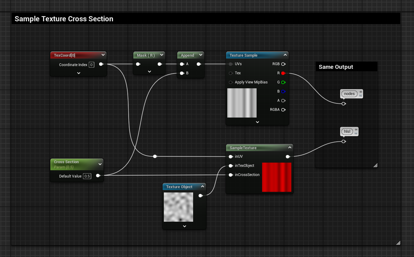
Sample Texture Cross Section in a Custom Node
I don’t write much code on a day-to-day basis, when doing something more complex than simple operations, it’s a good practice to break down what you are trying to achieve in isolated tests.
I started with a very simple test, by sampling the texture noise used for the cross-section, exactly in the same way I have shown before using generic nodes. If you want to know more about sampling textures in HLSL, check out this other post I’ve made → Sample Texture in HLSL
Here’s the code I’ve used to sample the texture:
// Sample Texture Cross Section
float myOut = Texture2DSample(inTexObject, inTexObjectSampler, float2(inUV.x, inCrossSection));
return myOut;
Segment SDF Function
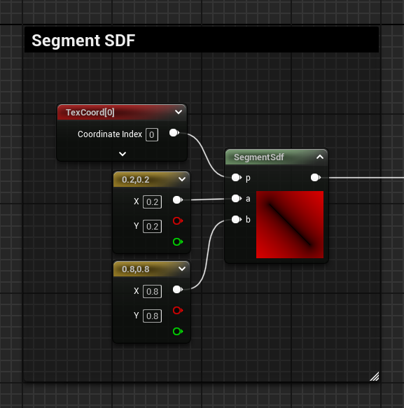
If you need SDFs, Inigo Quilez is your guy. Here’s the function for an SDF segment → 2D distance functions
I also wrote some stuff on this topic, specifically targeting it for Unreal Materials, check them out here if you are interested → 2D SDF – Basic Shapes and Visualization – Material Function Library
Here’s the code for the SDF function setup in a custom node:
float2 pa = p-a;
float2 ba = b-a;
float h = clamp( dot(pa,ba)/dot(ba,ba), 0.0, 1.0 );
return length( pa - ba*h );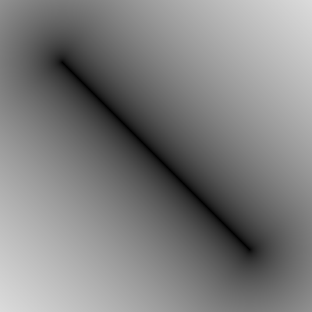
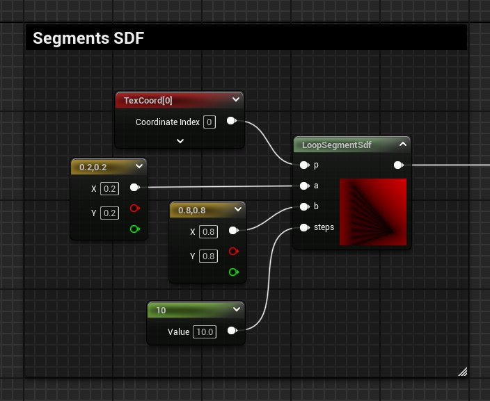
Segment SDF Function in a Loop
The next step was to get the logic wrapped in a loop, combine all the results and output the SDF.
To do that, I’ve made the loop, calculated a float value t, which represents the current loop integer index as a float normalised 0 to 1, and used it as the Y axis for one of the two point positions of the segment.
To combine all the segments, I’ve used a min operation and made sure the SDF initialized with a big value at the very start.
Here’s the code:
// SDF Function in a loop
float sdf = 1000000; //initialize with big number to allow for Min operation later

// Loop
for(int i = 0; i < steps; i++)
{
    float t = float(i) / float(steps - 1);  // Current loop i normalised 0 to 1
    float2 aNew = float2(a.x, t); // New a position using t for the Y axis

    // Segment SDF function
    float2 pa = p - aNew;
    float2 ba = b - aNew;
    float h = clamp( dot(pa,ba)/dot(ba,ba), 0.0, 1.0 );
    float l = length( pa - ba*h );
    sdf = min(sdf, l); // Combine current segment with the ones from the previous loop
}

return sdf;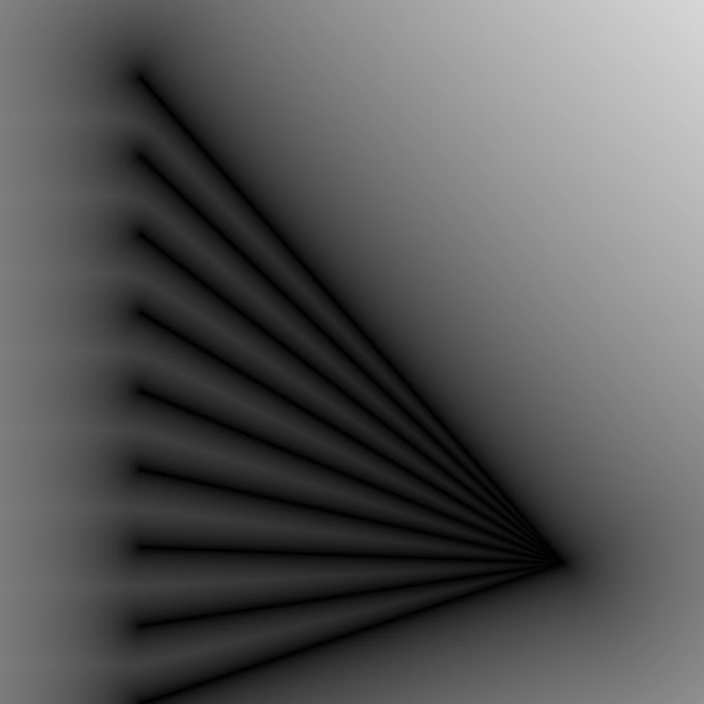
Circles
A segment SDF requires 2 positions, so to make it simpler, I first tried using the function of a circle, which only requires one position.
Here’s the code:
// Cross Section SDF Circles
float sdf = 1000000; //initialise with big number to allow for Min operation later

for(int i = 0; i < inSegments; i++)
{
    // Calculate current segment start and end positions (a and b)
    float t = float(i) / float(inSegments - 1); // Current loop i normalised 0 to 1
    float noise = Texture2DSample(inTexObject, inTexObjectSampler, float2(t, inCrossSection));   // Sample Texture with t and the input Cross Section target
    float2 a = float2(t, noise); // Set the position of the circle

    // Circle SDF function, offsets the UVs with the circle position centering it
    float l = length( inUV - a );

    sdf = min(sdf, l);    // Combine current segment with the ones from the previous loop
}

return sdf;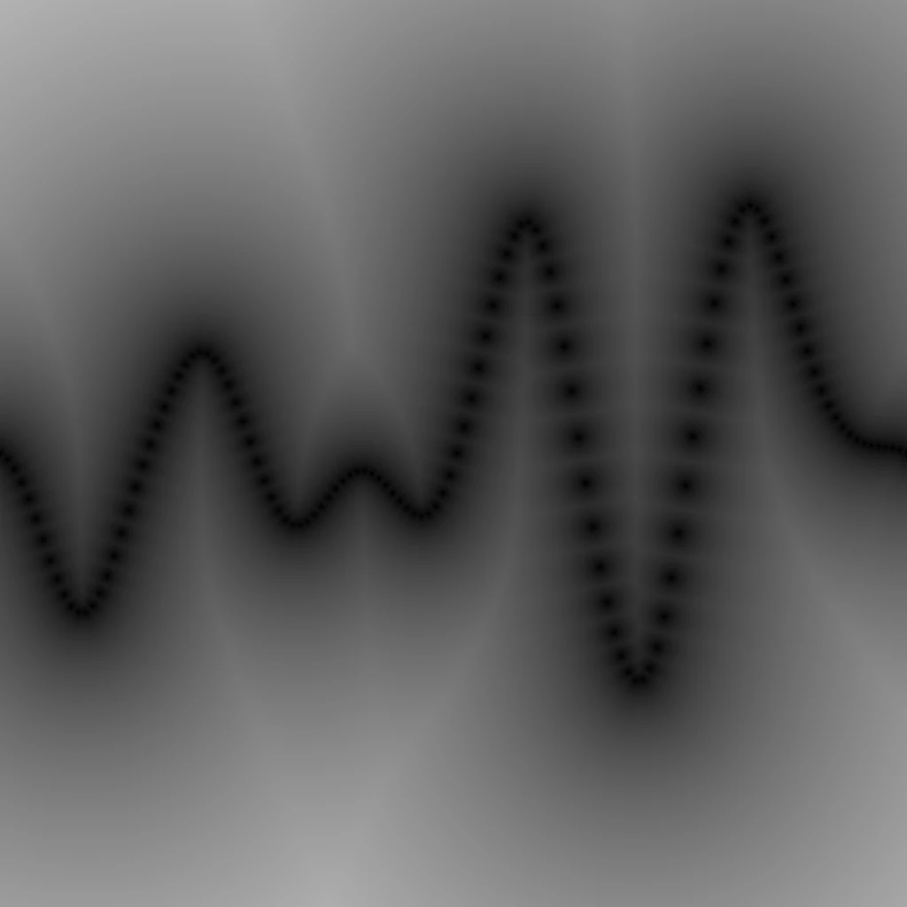
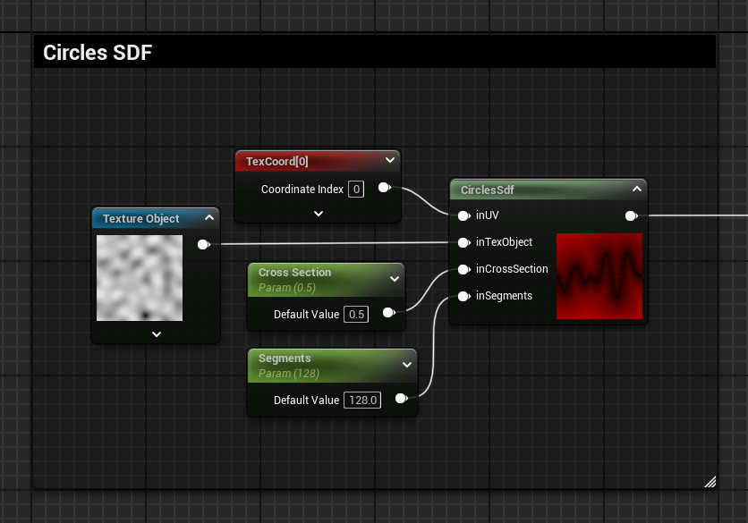
Here, you can start noticing the same behaviour examined before when investigating the FX-Map node in Substance Designer. The dots don’t look like they are equidistant from each other. Comparing only the U axis, they are, however, the sampled noise is applied on their V position, pushing them apart.
♪ All Together Now ♪
Then I’ve combined all these isolated tests.
Because the Segment SDF function expects 2 positions to draw the line, unfortunately I had to sample the texture twice for each iteration, one to fetch the Start point and another time for the End position. I don’t believe there is any way to store the End position during one iteration and re-use it as the Start position for the next iteration, so we are forced to sample the texture twice during each iteration.
I’ve replaced the circles SDF function with the segment one accordingly, by adding the additional texture sampler and the necessary variables for both start and end positions.
I also removed the “-1” applied to the input segments when t gets normalized, this way the output results in exactly the amount of segments fed as the value specified by the input float.
Here’s the code:
// Cross Section SDF Segments
float sdf = 1000000; //initialise with big number to allow for Min operation later

for(int i = 0; i < inSegments; i++)
{
    // Calculate current segment start and end positions (a and b)
    float tStart = float(i) / float(inSegments); // Current loop i normalised 0 to 1
    float tEnd = float(i + 1) / float(inSegments); // Previous loop i normalised 0 to 1
    float noiseStart = Texture2DSample(inTexObject, inTexObjectSampler, float2(tStart, inCrossSection));   // Sample Texture with t and the input Cross Section target
    float noiseEnd = Texture2DSample(inTexObject, inTexObjectSampler, float2(tEnd, inCrossSection));   // Sample Texture with t and the input Cross Section target
    float2 a = float2(tStart, noiseStart); // Segment Start Position
    float2 b = float2(tEnd, noiseEnd); // Segment End Position

    // Segment SDF function
    float2 pa = inUV - a;
    float2 ba = b - a;
    float h = clamp( dot(pa,ba)/dot(ba,ba), 0.0, 1.0 );
    float l = length( pa - ba*h );

    sdf = min(sdf, l);    // Combine current segment with the ones from the previous loop
}

return sdf;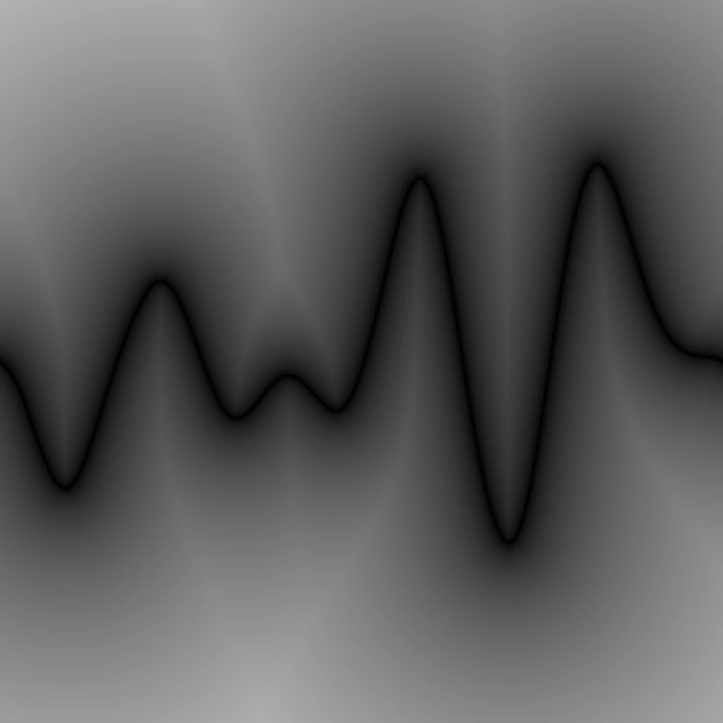
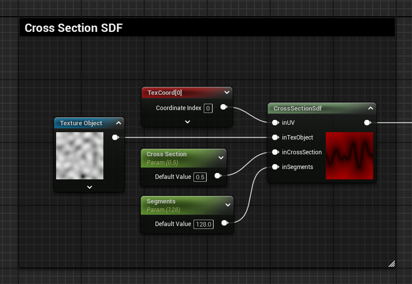
I tried to keep it simple, so I’ve only supported one axis in this setup, but you can, of course, expand on it with what was shown earlier in the post.
Keep in mind that these can be expensive operations, especially if you set a high count of segments. It’s not really something I would use in a project, other than in very specific cases.
I can’t think of many use case examples that might require something like this. Most of the time, you could get away by simply baking the result to a static texture. The only cool thing about this setup is that it’s calculated dynamically, so the cross-section can be animated!
One fun example where this might be a useful setup for, could be if you’re making a dynamic waveform FX that needs to react to an audio input.
Some Fun
These exploration posts take me so long to write and prepare, when I reached this point and had it almost ready to published I decided to try and have some more fun. I got this far, might as well squeeze in something extra.
I wasn’t really sure what I wanted to achieve; I just wanted to try and combine some waves and see what I could get.
Offset UVs
The first thing I thought of was adding some motion using UV offset; however, when adding an offset of 0.5, I noticed a flaw in the setup.
The SDF segments are only drawn in the 0-1 range of the UVs, so a frac operation needs to be introduced. However, this is still not enough; a visible seam is present where the texture tiles. This is because there are no segments generated beyond the 0-1 range, and the SDF is generated accordingly, as if there is nothing beyond that point, because there isn’t.
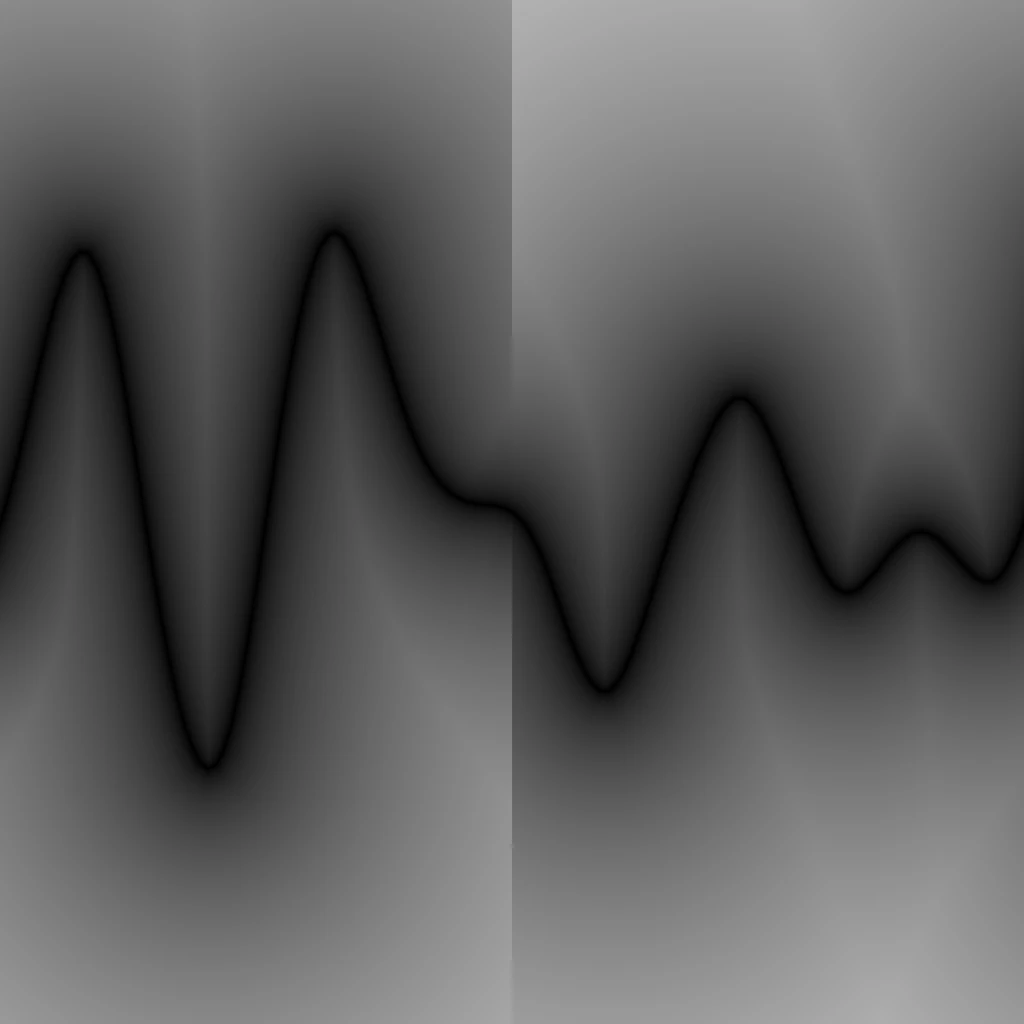
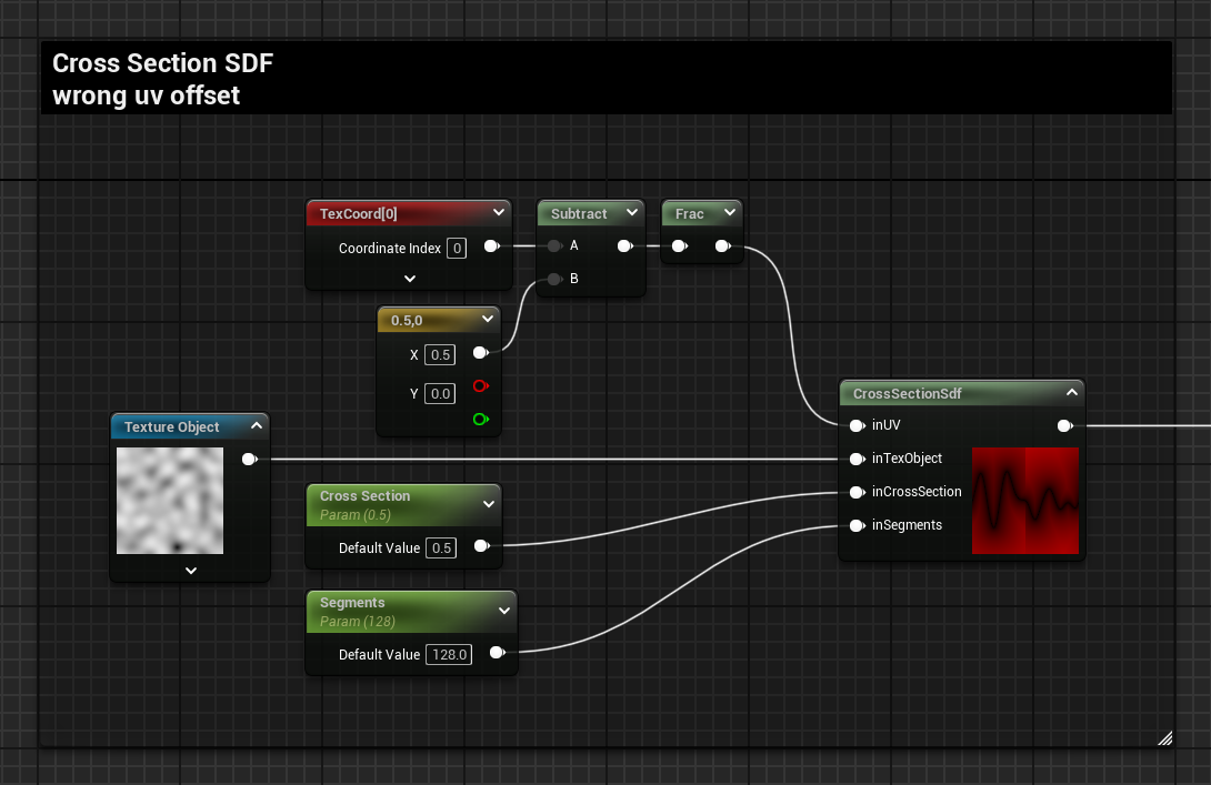
The UV input is only used for the sampling of the SDF, instead of adding an offset to these UVs, the offset can be added to the positions of the segments when sampling the texture.
A new input is added to the Custom node, inOffset, and here’s the 2 lines of code that need to be updated:
float noiseStart = Texture2DSample(inTexObject, inTexObjectSampler, float2(tStart, inCrossSection) - inOffset);
    float noiseEnd = Texture2DSample(inTexObject, inTexObjectSampler, float2(tEnd, inCrossSection) - inOffset);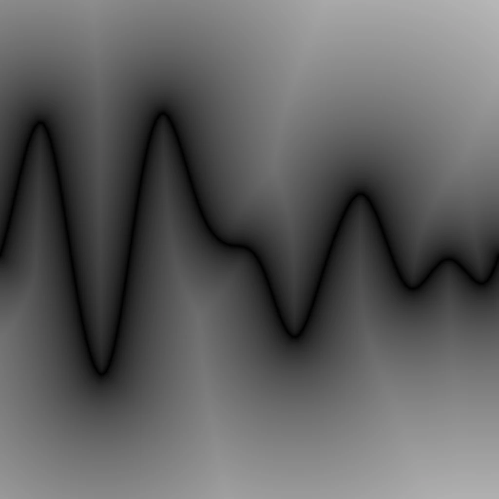

More Controls and 2 Waves Combined
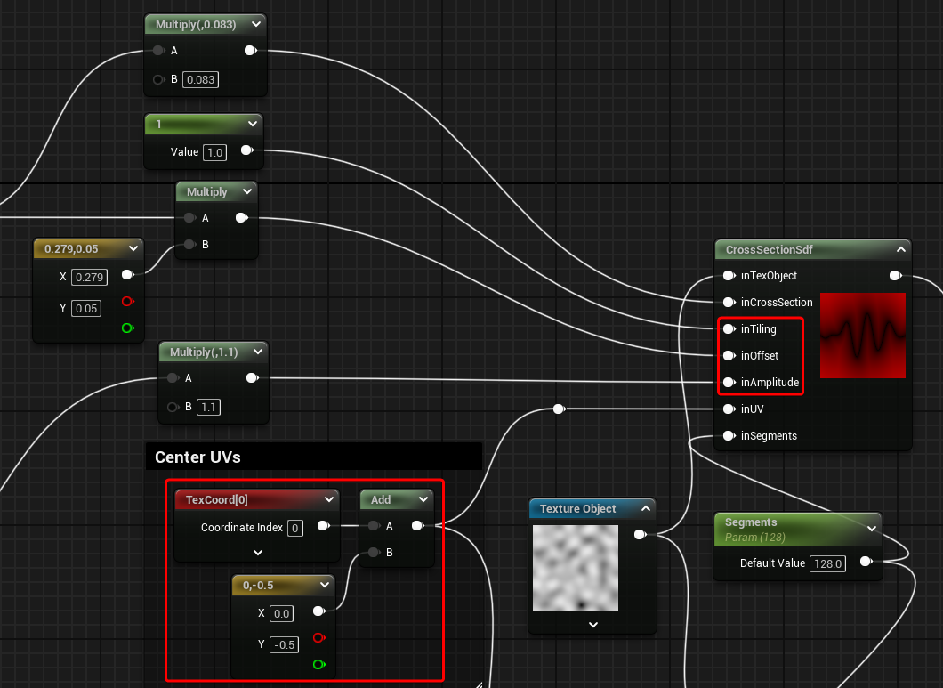
I started trying to duplicate my custom node and have 2 waves combined. I’ve quickly realised that I didn’t have enough control to do what I wanted. I’ve proceeded with exposing the Offset parameter, but also implemented control over the Amplitude and Tiling in the same way (manipulating the segments positions).
To note, in order for the amplitude to work as expected, I’ve also had to centre the UVs, for both the field used by the SDF as well as offsetting the start and end positions of the segments.
Here’s the graph and the HLSL code of the updated function:
// Cross Section SDF Segments
float sdf = 1000000; //initialise with big number to allow for Min operation later

for(int i = 0; i < inSegments; i++)
{
    // Calculate current segment start and end positions (a and b)
    float tStart = float(i) / float(inSegments); // Current loop i normalised 0 to 1
    float tEnd = float(i + 1) / float(inSegments); // Previous loop i normalised 0 to 1

    // Sample Textures with t and the input Cross Section target, also applying tiling, offset and amplitude
    float noiseStart = Texture2DSample(inTexObject, inTexObjectSampler, (float2(tStart, inCrossSection) * inTiling) - inOffset);   // Texture Sample Segment Start
    float noiseEnd = Texture2DSample(inTexObject, inTexObjectSampler, (float2(tEnd, inCrossSection) * inTiling) - inOffset);   // Texture Sample Segment End
    noiseStart += -0.5; //Centers Segments Positions (UVs are now also centered)
    noiseEnd += -0.5; //Centers Segments Positions (UVs are now also centered)
    noiseStart *= inAmplitude; // Previous step now allows exposing amplitude
    noiseEnd *= inAmplitude; // Previous step now allows exposing amplitude

    // Start and End Positions for the segment SDF
    float2 a = float2(tStart, noiseStart); // Segment Start Position
    float2 b = float2(tEnd, noiseEnd); // Segment End Position

    // Segment SDF function
    float2 pa = inUV - a;
    float2 ba = b - a;
    float h = clamp( dot(pa,ba)/dot(ba,ba), 0.0, 1.0 );
    float l = length( pa - ba*h );

    sdf = min(sdf, l);    // Combine current segment with the ones from the previous loop
}

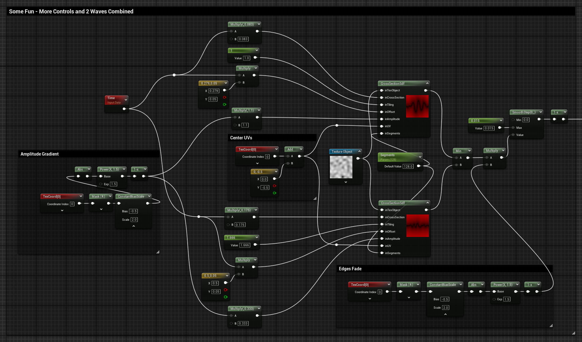
return sdf;Below you can see what I came up with; it’s just a bunch of random values for the various parameters, with two waves of different frequencies. I’ve also scaled the SDF at the edges, making it look like the waves are expanding.
Final result and graph:
2 Textures Combined in 1 Output
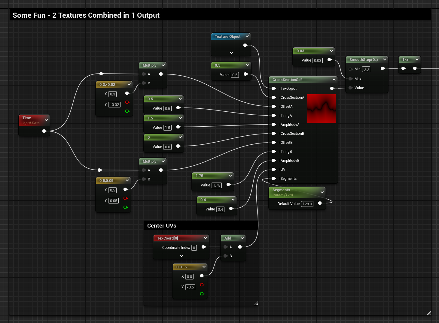
I’ve then expanded the custom node so that it can sample the texture 2 times and combined their cross sections before sampling the SDF.
The result:
The graph:
And here’s the code if you are interested:
// Cross Section SDF Segments
float sdf = 1000000; //initialise with big number to allow for Min operation later

for(int i = 0; i < inSegments; i++)
{
    // Calculate current segment start and end positions (a and b)
    float tStart = float(i) / float(inSegments); // Current loop i normalised 0 to 1
    float tEnd = float(i + 1) / float(inSegments); // Previous loop i normalised 0 to 1

    // Sample the First Noise: A
    // Sample Textures with t and the input Cross Section target, also applying tiling, offset and amplitude
    float noiseStartA = Texture2DSample(inTexObject, inTexObjectSampler, (float2(tStart, inCrossSectionA) * inTilingA) - inOffsetA); // Texture Sample Segment Start
    float noiseEndA = Texture2DSample(inTexObject, inTexObjectSampler, (float2(tEnd, inCrossSectionA) * inTilingA) - inOffsetA); // Texture Sample Segment End
    noiseStartA += -0.5; //Centers Segments Positions (UVs are now also centered)
    noiseEndA += -0.5; //Centers Segments Positions (UVs are now also centered)
    noiseStartA *= inAmplitudeA; // Previous step now allows exposing amplitude
    noiseEndA *= inAmplitudeA; // Previous step now allows exposing amplitude

    // Sample the Second Noise: B
    // Sample Textures with t and the input Cross Section target, also applying tiling, offset and amplitude
    float noiseStartB = Texture2DSample(inTexObject, inTexObjectSampler, (float2(tStart, inCrossSectionA) * inTilingB) - inOffsetB); // Texture Sample Segment Start
    float noiseEndB = Texture2DSample(inTexObject, inTexObjectSampler, (float2(tEnd, inCrossSectionA) * inTilingB) - inOffsetB); // Texture Sample Segment End
    noiseStartB += -0.5; //Centers Segments Positions (UVs are now also centered)
    noiseEndB += -0.5; //Centers Segments Positions (UVs are now also centered)
    noiseStartB *= inAmplitudeB; // Previous step now allows exposing amplitude
    noiseEndB *= inAmplitudeB; // Previous step now allows exposing amplitude

    // Combine the 2 sampled noises, scales down to keep in range when default of 1 is used
    float noiseStart = (noiseStartA + noiseStartB) * 0.5;
    float noiseEnd = (noiseEndA + noiseEndB) * 0.5;

    // Start and End Positions for the segment SDF
    float2 a = float2(tStart, noiseStart); // Segment Start Position
    float2 b = float2(tEnd, noiseEnd); // Segment End Position

    // Segment SDF function
    float2 pa = inUV - a;
    float2 ba = b - a;
    float h = clamp( dot(pa,ba)/dot(ba,ba), 0.0, 1.0 );
    float l = length( pa - ba*h );

    sdf = min(sdf, l);    // Combine current segment with the ones from the previous loop
}

return sdf;Conclusion
Thanks for reaching this point!
This was a really fun exploration to do, even though I didn’t really reach the “100% useful outcome” I was hoping for.
I believe the Pseudo SDF Gradient technique is extremely useful since I’ve been using it almost on a daily basis to debug what a gradient looks like; however, with this exploration, I was hoping to find a nice and cheap way to draw curves with uniform thickness, but the HLSL for loop cost is not really that justifiable to be used for extensive use.
I also thought about looking into a way of reducing the iterations required by having fewer segments and creating the smooth curvature by calculating Bézier SDFs, which would give an approximated, but smooth result. It would have been fun just to try it out, but I’ve already spent enough time on this.
I hope it was an enjoyable and insightful read, until the next one!
Resources
- SDF segment → 2D distance functions
- Substance Designer
- FX-Map Documentation → FX-Map | Substance 3D Designer
- FX Map basics → Tutorial – Substance Designer FX Map Basics
Leave a Reply